AIモデルを用いた画像分類による鋳造製品の品質判定アプリ

このブログはAidemy Premiumのカリキュラムの一環で、受講修了条件を満たすために公開しています

はじめに

私は、これまでソフトウェア業界でパッケージソフトウェアの導入コンサルタントや海外SaaSのカスタマーサクセスといった営業職経験者です。

パッケージソフトウェアやAPI,海外SaaSを導入する業務範囲で必要となるシステム知識やSQL(データ操作言語のみ)の経験と独学でPythonやGoに触れたことある程度でAIアプリの作成に取り組みました。

本記事の概要

• Pythonを用い画像分類モデルを作成し、ウェブアプリケーションに実装した過程について記載
• 今回は、鋳造製品の表のみを対象に画像で異常と正常を分類するモデルを作成
• 教師あり学習(分類)、転移学習、CNN、Flaskなどについて記載

作成したアプリケーション

以下のリンクより作成したWebアプリケーションにアクセスできます。
鋳造製品の表面における異常、正常判定アプリ

目次

1. 作業フロー
2. 実行環境
3. 画像収集
4. 機械学習モデルの作成・実行
5. ウェブアプリケーション作成
6. 結果と考察
7. 今後の活用
8. おわりに
9. 参考記事

1.作業フロー

順番	概要	詳細
1	テーマ検討	作成するアプリの方向性を検討。今回は画像を分類するモデルを実装したアプリを作成しました。
2	画像収集	学習に使うための画像を収集。今回は、Kaggleからダウンロードしました。
3	機械学習モデルの作成	AIアプリ開発コース内で学習した男女識別のモデルを参考にしました。
4	モデルのテスト、評価	テストを実施し、精度とファイルサイズの調整を繰り返し、適切なモデルを作成。
5	クライアントサイドとサーバーサイドの処理	ウェブアプリケーションとして動作させるための処理を用意。
6	デプロイ	作成したモデルを実行するアプリをローカルではなく一般的に利用できるように公開します。

2. 実行環境

• MacBookPro M3
• macOS Sonama 14.5
• モデル構築：
  • 言語：Python 3.11.5
  • 使用サービス：Google Colaboratory
• Webページデザイン：
  • 言語：html, css,
  • ウェブフレームワーク：Flask 2.2.2
  • 使用サービス：Visual Studio Code
• アプリのデプロイ：
  • 使用サービス：ターミナル、GitHub, Render

3.画像収集

画像は、Kaggleの以下ページより異常:781枚、正常:519枚をダウンロード後、Google Colaboratoryに保存し使用しました。

casting product image data for quality inspection

4. 機械学習モデルの作成・実行

ライブラリをインポート

必要となるライブラリをインポートします。
画像分類を得意としているものやグラフ描画のライブラリを選択します。

ライブラリインポート

import os
import cv2
import numpy as np
import matplotlib.pyplot as plt
from tensorflow.keras.utils import to_categorical
from tensorflow.keras.layers import Dense, Dropout, Flatten, Input
from tensorflow.keras.applications.vgg16 import VGG16, preprocess_input
from tensorflow.keras.models import Model, Sequential
from tensorflow.keras.optimizers import Adam
from sklearn.metrics import recall_score, precision_recall_curve, average_precision_score
import json
import keras.backend as K
import shap

• osモジュール
  • OSに依存しているさまざまな機能を利用するためのモジュール。ファイルやディレクトリ関係の操作の際に利用
• OpenCV (cv2) ライブラリ
  • 画像の読み込み、前処理、または操作に使用
• NumPy (np) ライブラリ
  • 画像を数値配列として表現し、Pythonで処理するため
• Matplotlib ライブラリのプロットモジュール
  • 画像や訓練結果（損失曲線、精度プロットなど）を可視化
• TensorFlow Keras utils モジュールの to_categorical 関数をインポート
  • カテゴリカルラベルをワンホットエンコーディングするため

画像取り込み

今回画像ファイルは、google driveに保存したのでマウントを行いました。

マウント

from google.colab import drive
drive.mount('/content/drive')

画像の調整

リサイズの処理を追加しました。
オリジナルサイズの512で実施したときは、モデルファイルが700MBを超え処理が遅くなってしまったので、100MB以下で良い大きさになるよう調整をしました。
また、学習に用いた画像の枚数が異常と正常で異なる状態で実施したものを最終的には500に揃えモデル化しました。

実施した内容

1. 画像を指定されたパスから読み込む
2. 画像の色空間をBGRからRGBに変換
3. 画像データを float32 型に変換し、0から1の範囲に正規化
4. 画像のサイズを指定されたサイズにリサイズ
5. 前処理された画像をリストに追加

事前準備

# Load images
path_def_front = os.listdir('/content/drive/MyDrive/Aidemy_Projectfolder/images/def/')
path_ok_front = os.listdir('/content/drive/MyDrive/Aidemy_Projectfolder/images/ok/')

img_def_front = []
img_ok_front = []
imgsize = 150

for i in range(len(path_def_front)):
    img_path = os.path.join('/content/drive/MyDrive/Aidemy_Projectfolder/images/def/' + path_def_front[i])
    img = cv2.imread(img_path)
    img = cv2.cvtColor(img, cv2.COLOR_BGR2RGB)
    img = img.astype(np.float32) / 255.0
    img = cv2.resize(img, (imgsize, imgsize))
    img_def_front.append(img)

for i in range(len(path_ok_front)):
    img_path = os.path.join('/content/drive/MyDrive/Aidemy_Projectfolder/images/ok/' + path_ok_front[i])
    img = cv2.imread(img_path)
    img = cv2.cvtColor(img, cv2.COLOR_BGR2RGB)
    img = img.astype(np.float32) / 255.0
    img = cv2.resize(img, (imgsize, imgsize))
    img_ok_front.append(img)

X = np.array(img_def_front + img_ok_front)
y = np.array([0]*len(img_def_front) + [1]*len(img_ok_front))

# Shuffle data
rand_index = np.random.permutation(len(X))
X, y = X[rand_index], y[rand_index]

# Split data
split_index = int(len(X) * 0.8)
X_train, X_test = X[:split_index], X[split_index:]
y_train, y_test = y[:split_index], y[split_index:]

y_train = to_categorical(y_train, num_classes=2)
y_test = to_categorical(y_test, num_classes=2)

学習内容の設定

ハイパーパラメータなどを設定します。
今回は、VGG16という「ImageNet」と呼ばれる大規模画像データセットで学習された16層からなるCNNモデルを使って転移学習を行いました。

学習用データとテストデータを読み込み、ラベルのOne-hot表現などをします。
One-hot表現とは、ダミー変数を用いて正解ラベルを1、それ以外を0にすることです。

モデルの構築・学習の際に、ハイパーパラメータ（人が決める数値）である、batch_size, epochs（試行回数）等を調整します。

その他データ処理

# Model setup
input_tensor = Input(shape=(imgsize, imgsize, 3))
vgg16 = VGG16(include_top=False, weights='imagenet', input_tensor=input_tensor)

top_model = Sequential()
top_model.add(Flatten(input_shape=vgg16.output_shape[1:]))
top_model.add(Dense(256, activation='relu'))
top_model.add(Dropout(0.5))
top_model.add(Dense(2, activation='softmax'))

model = Model(vgg16.inputs, top_model(vgg16.output))

for layer in model.layers[:19]:
    layer.trainable = False

model.compile(optimizer='adam', loss='binary_crossentropy', metrics=['accuracy'])

# Model training
history = model.fit(X_train, y_train, batch_size=50, epochs=30, validation_data=(X_test, y_test))

SDGでテストしたときは、最高70%程度のaccuracyでした。
SDGからadamに変更したら大幅に精度が向上しました。
画像サイズが512のときには、以下の結果になりました。

モデルのテストや評価

def casting_defect(img):
    img = cv2.resize(img, (imgsize, imgsize))
    pred = np.argmax(model.predict(np.array([img])))
    if pred == 0:
        return 'def_front'
    else:
        return 'ok_front'

scores = model.evaluate(X_test, y_test, verbose=1)
print('Test loss:', scores[0])
print('Test accuracy:', scores[1])

y_test_pred = model.predict(X_test)
y_test_pred_classes = np.argmax(y_test_pred, axis=1)
y_test_true_classes = np.argmax(y_test, axis=1)
recall = recall_score(y_test_true_classes, y_test_pred_classes)
print('Test recall:', recall)

y_pred_proba = model.predict(X_test)
precision, recall, thresholds = precision_recall_curve(y_test[:, 1], y_pred_proba[:, 1])
average_precision = average_precision_score(y_test[:, 1], y_pred_proba[:, 1])

plt.figure()
plt.step(recall, precision, color='b', alpha=0.2, where='post')
plt.fill_between(recall, precision, step='post', alpha=0.2, color='b')
plt.xlabel('Recall')
plt.ylabel('Precision')
plt.ylim([0.0, 1.05])
plt.xlim([0.0, 1.0])
plt.title(f'Precision-Recall curve: AP={average_precision:.2f}')
plt.show()

train_loss = history.history['loss']
val_loss = history.history['val_loss']
acc = history.history["accuracy"]
val_acc = history.history["val_accuracy"]
epochs = len(train_loss)

fig = plt.figure(figsize=(15,5))
plt.subplots_adjust(wspace=0.4, hspace=0.6)
ax1 = fig.add_subplot(1,2,1)
ax1.plot(range(epochs), train_loss, marker = '.', label = 'train_loss')
ax1.plot(range(epochs), val_loss, marker = '.', label = 'val_loss')
ax1.legend(loc = 'best')
ax1.set_xlabel('epoch')
ax1.set_ylabel('loss')

ax2 = fig.add_subplot(1,2,2)
ax2.plot(range(epochs), acc, label="acc", ls="-", marker=".")
ax2.plot(range(epochs), val_acc, label="val_acc", ls="-", marker=".")
ax2.set_ylabel("accuracy")
ax2.set_xlabel("epoch")
ax2.legend(loc="best")

plt.show()

y_pred = model.predict(X_test)[:, 1]
y_pred = (y_pred > 0.5).astype(int)
precision, recall, thresholds = precision_recall_curve(y_test[:, 1], y_pred)

plt.plot(recall, precision, thresholds)
plt.xlabel("Recall")
plt.ylabel("Precision")
plt.title("PR Curve")
plt.show()

img = cv2.imread('/content/drive/MyDrive/Aidemy_Projectfolder/images/def/' + path_def_front[0])
b, g, r = cv2.split(img)

img1 = cv2.merge([r, g, b])

plt.imshow(img1)
plt.show()
print(casting_defect(img))

explainer = shap.GradientExplainer(model, preprocess_input(X_test.copy()))

# テストセットの最初の5つの画像に対してSHAP値を計算
shap_values = explainer.shap_values(preprocess_input(X_test[:5].copy()))

# 各クラスの名前
class_names = ['def_front', 'ok_front']

# SHAP値のプロット
for i in range(5):
    # 画像データを0〜1の範囲にクリップ
    X_test_clipped = np.clip(X_test[i:i+1], 0, 1)
    shap.image_plot(shap_values, X_test_clipped, class_names)
    X_test_scaled = (X_test_clipped - X_test_clipped.min()) / (X_test_clipped.max() - X_test_clipped.min())

# Visualization of misclassified images
misclassified = []
cnt = 0
plt.figure(figsize=(20, 8))
test_cases = [('/content/drive/MyDrive/Aidemy_Projectfolder/images/def/' + i, 'def') for i in path_def_front] + \
             [('/content/drive/MyDrive/Aidemy_Projectfolder/images/ok/' + i, 'ok') for i in path_ok_front]

for img_path, actual_label in test_cases:
    if cnt == 10:
        break  # show max 10 images
    img = cv2.imread(img_path)
    img_resized = cv2.resize(img, (imgsize, imgsize)).astype(np.float32) / 255.0
    prediction = model.predict(np.expand_dims(img_resized, axis=0))
    predicted_label = 'def' if np.argmax(prediction) == 0 else 'ok'

    if predicted_label != actual_label:
        misclassified.append((img_path, actual_label, predicted_label))
        plt.subplot(2, 5, cnt + 1)
        plt.title(f"{os.path.basename(img_path)}\n Actual Label: {actual_label}", weight='bold', size=12)
        cv2.putText(img=img, text=f"Predicted Label: {predicted_label}", org=(10, 30), fontFace=cv2.FONT_HERSHEY_SIMPLEX,
                    fontScale=0.8, color=(255, 0, 255), thickness=2)
        cv2.putText(img=img, text=f"Probability: {'{:.3f}'.format(prediction[0][np.argmax(prediction)] * 100)}%", org=(10, 280),
                    fontFace=cv2.FONT_HERSHEY_SIMPLEX, fontScale=0.7, color=(0, 255, 0), thickness=2)
        plt.imshow(cv2.cvtColor(img, cv2.COLOR_BGR2RGB))
        plt.axis('off')
        cnt += 1

plt.show()

実施内容

1. テスト用関数の作成
2. モデルの評価
3. 再現率の計算
4. PR曲線のプロット
5. トレーニング過程の可視化

最終的な精度

Epoch 30/30
loss: 0.1513 - accuracy: 0.9380 - val_loss: 0.1302 - val_accuracy: 0.9703
loss: 0.1302 - accuracy: 0.9703

Test loss: 0.13017480075359344
Test accuracy: 0.9702970385551453
Test recall: 0.963302752293578

ハイパーパラメータなどを調整している段階では、さほど影響がありませんでしたが、shapなどのために処理を追加し始めてから99%に到達した正解率も90%中盤まで下がりました。

うまくできませんでしたが、shapで予測結果の説明を試みました。
正解率と再現率が高い数値のためその結果の実態を確認するために取り組みました。

shapとは

SHAP (SHapley Additive exPlanations)を用いて、2つの画像の分類における特徴の影響を可視化するものです。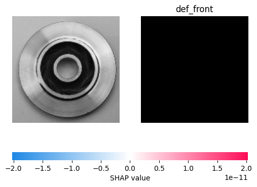

画像内に予測ラベルと確率を可視化

# casting_defect関数に鋳造の写真を渡して正常性を判定します
img = cv2.imread('/content/drive/MyDrive/Aidemy_Projectfolder/images/def/' + path_def_front[0])
b,g,r = cv2.split(img)
img1 = cv2.merge([r,g,b])
plt.imshow(img1)
plt.show()
print(casting_defect(img))



#resultsディレクトリを作成
result_dir = 'results'
if not os.path.exists(result_dir):
    os.mkdir(result_dir)

#モデルを保存。
model.save('casting_defect_model1_4.h5')

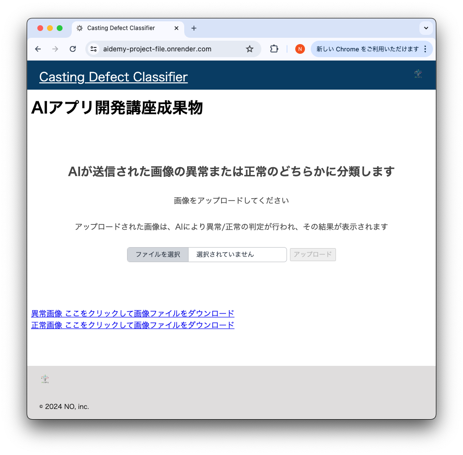
5. ウェブアプリケーション作成

HTML,CSS,Flaskを作成し、ターミナルを用いて、GitHubとRenderでデプロイします。

クライアントサイド

HTMLコード

<!DOCTYPE html>
<html lang="ja">
<head>
    <meta charset="UTF-8">
    <meta name="viewport" content="width=device-width, initial-scale=1.0">
    <meta http-equiv="X-UA-Compatible" content="ie=edge">
    <title>Casting Defect Classifier</title>
    <link rel="stylesheet" href="./static/stylesheet.css">
    <link rel="icon" href="./static/favicon.ico" type="image/x-icon">
</head>
<body>
    <header>   
        <img class="header_img" src="https://aidemyexstorage.blob.core.windows.net/aidemycontents/1621500180546399.png" alt="Aidemy">
        <a class="header-logo" href="#">Casting Defect Classifier</a>
    </header>
    <div class="main">
        <h1>AIアプリ開発講座成果物</h1>
        <h2>AIが送信された画像の異常または正常のどちらかに分類します</h2>
        <p>画像をアップロードしてください</p>
        <p>アップロードされた画像は、AIにより異常/正常の判定が行われ、その結果が表示されます</p>
        <form id="uploadForm" method="post" enctype="multipart/form-data">
          <input type="file" id="fileInput" name="fileInput">
          <button type="submit" id="uploadButton" disabled>アップロード</button>
        </form>
        <div class="answer">{{answer}}</div>
        <br>
        <a href="https://drive.google.com/file/d/view?usp=drive_link" download>異常画像 ここをクリックして画像ファイルをダウンロード</a>
        <br>
        <a href="https://drive.google.com/file/d/1wEhfq1mfI0SYfxV1h-view?usp=drive_link" download>正常画像 ここをクリックして画像ファイルをダウンロード</a>  
    </div>
    <footer>
        <img class="footer_img" src="https://aidemyexstorage.blob.core.windows.net/aidemycontents/1621500180546399.png" alt="Aidemy">
        <small>&copy; 2024 NO, inc.</small>
    </footer>

    <script>
        document.addEventListener('DOMContentLoaded', function () {
        const fileInput = document.getElementById('fileInput');
        const uploadButton = document.getElementById('uploadButton');
          fileInput.addEventListener('change', function () {
          if (fileInput.files.length > 0) {
              uploadButton.disabled = false;
          } else {
              uploadButton.disabled = true;
              }
          });
        });
    </script>
</body>
</html>

工夫した点

• ファビコンを設定
• ファイルが未選択のときは、アップロードボタンが無効になるJavaScriptを追加

CSSコード

header {
    background-color: #093c63;
    height: 60px;
    margin: -8px;
    display: flex;
    flex-direction: row-reverse;
    justify-content: space-between;
    font-family: 'Noto Sans JP', sans-serif;
}

.header-logo {
    color: #fff;
    font-size: 25px;
    margin: 15px 25px;
}

.header_img {
    height: 25px;
    margin: 15px 25px;
}

.main {
    height: 370px;
    font-family: 'Noto Sans JP', sans-serif;
}

h2 {
    color: #444444;
    margin: 90px 0px 30px 0px;
    text-align: center;
    font-family: 'Noto Sans JP', sans-serif;
}

p {
    color: #444444;
    margin: 30px 0px 30px 0px;
    text-align: center;
    font-family: 'Noto Sans JP', sans-serif;
}

.answer {
    color: #444444;
    margin: 70px 0px 30px 0px;
    text-align: center;
    font-family: 'Noto Sans JP', sans-serif;
}

form {
    text-align: center;
    font-family: 'Noto Sans JP', sans-serif;
}

footer {
    background-color: #dfdddd;
    height: 110px;
    left: 0;
    bottom: 0;
    width: 100%;
    position: fixed;
    font-family: 'Noto Sans JP', sans-serif;
}

.footer_img {
    height: 25px;
    margin: 15px 25px;
}

small {
    margin: 15px 25px;
    position: absolute;
    left: 0;
    bottom: 0;
    font-family: 'Noto Sans JP', sans-serif;
}
input[type='file'] {
  color: rgb(31, 41, 55);
  cursor: pointer;
  border: 1px solid rgb(191, 194, 199);
  border-radius: 0.375rem;
  padding-right: 0.5rem;
  width: 20rem;
}

::file-selector-button,
::-webkit-file-upload-button {
  background-color: rgb(209, 213, 219);
  color: rgb(31, 41, 55);
  border: none;
  cursor: pointer;
  border-right: 1px solid rgb(191, 194, 199);
  padding: 0.25rem 1rem;
  margin-right: 1rem;
}
input[type='submit'] {
  color: rgb(31, 41, 55);
  cursor: pointer;
  border: 1px solid rgb(191, 194, 199);
  border-radius: 0.375rem;
  padding-right: 0.5rem;
  width: 10rem;
}

ファイル選択のフォームのデザインを少し変えました。

サーバーサイド

Flask

import os
from flask import Flask, request, redirect, render_template, flash
from werkzeug.utils import secure_filename
from tensorflow.keras.models import Sequential, load_model
from tensorflow.keras.preprocessing import image

import numpy as np



# ねじれ:classes = ["正常","異常"]
classes = ["異常","正常"]
image_size = 150

UPLOAD_FOLDER = "uploads"
ALLOWED_EXTENSIONS = set(['png', 'jpg', 'jpeg', 'gif'])

app = Flask(__name__)

def allowed_file(filename):
    return '.' in filename and filename.rsplit('.', 1)[1].lower() in ALLOWED_EXTENSIONS

model = load_model('./casting_defect_model1_4.h5')#学習済みモデルをロード


@app.route('/', methods=['GET', 'POST'])
def upload_file():
    if request.method == 'POST':
        if 'fileInput' not in request.files:
            flash('ファイルがありません')
            return redirect(request.url)
        file = request.files['fileInput']
        if file.filename == '':
            flash('ファイルがありません')
            return redirect(request.url)
        if file and allowed_file(file.filename):
            filename = secure_filename(file.filename)
            file.save(os.path.join(UPLOAD_FOLDER, filename))
            filepath = os.path.join(UPLOAD_FOLDER, filename)

            #受け取った画像を読み込み、np形式に変換
            # 今回モデルはグレースケール指定ではないため、color_mode="grayscale"無指定
            img = image.load_img(filepath, target_size=(image_size,image_size))
            img = image.img_to_array(img)
            data = np.array([img])
            #変換したデータをモデルに渡して予測する
            result = model.predict(data)[0]
            predicted = result.argmax()
            pred_answer = "アップロードされた画像は、 " + classes[predicted] + " な製品画像です"
            return render_template("index.html",answer=pred_answer)
    return render_template("index.html",answer="")


if __name__ == "__main__":
    port = int(os.environ.get('PORT', 8080))
    app.run(host ='0.0.0.0',port = port)

ファイル選択前の画面

ファイルアップロード後の画面

6. 結果と考察

全体

モデルとアプリどちらもシンプルな内容でしたが、意図した結果が出力される画像のアプリを作成することができ安心しました。

モデル作成

鋳造製品の異常/正常を画像で分類するAIモデルを転移学習を用いて作成。
初期こそ正解率が70％程度でしたが、調整後は90％後半を維持できました。ただ利用状況を製品のチェックで使う場合再現率も重要になると考え後半は、PR曲線に取り組みました。
今回の画像データでは、再現率の数値も高いことがわかりました。
そこで、予測結果の説明ができる処理の追加を試みましたが力不足でうまくできませんでした。
評価の行いやすさも考慮できるようになる必要性を実感しました。

また、モデル作成時のaccuracyは90%以上にもかかわらず、アプリで画像をアップロードすると結果が意図した結果と逆転する事象が発生。
目的変数の順序とバックエンド処理のclassingの順序が一致しいていないことが原因。重要な接続部分の理解が不足しておりました。

アプリ作成

ファビコンをつけてみたり、フッターの位置をウィンドウサイズが変わっても下部に固定するなど参考にしたコードから軽微な修正。

flaskとhtmlの記述が一致していないため、途中でInternal errorが発生するなど、理解不足を改めて認識した。

7. 今後の活用

データについては、前処理をほとんどしていないので、その点について、復習する必要があると考えています。
また、データ量をなるべく揃えた状態で学習を実施したが、異常側のデータが少ない場合のモデル学習を行う必要がある場合の進め方にも興味を持ちました。
最小単位のサービスが作成できたので、ここから拡張していくもしくは、安定して運用していく、そしてセキュリティ面の確保など必須な領域についても取り組みたいと思います。

1つの成果物を作成することはできましたが、すべての理解度が低い状態です。少しずつ処理を追加していくにつれて目で見える成果物は、意図したものに近づく一方で、コードの内容を把握しきれなくなっている部分がありました。基礎の理解に時間を費やしたいと思います。
また、今回のゴールを自分で線引することができるものですが、要件とスケジュールに柔軟に対応できる技術や知識を身に着けて行きたいと思います。

8.おわりに

エラーが発生した際や少し工夫をしたいときには、過去のドキュメントやチューターの方に助けていただき進めることができました。ありがとうございます。

成果物作りは、とても楽しかったです。
既にあるものを参考としながらではありましたが、改善するための試行錯誤をする工程に充実感がありました。徐々に知識が広がり、やりたい事が増えて行く過程を楽しむことができました。
今後、個人でも開発を続けたいと思います。

9. 参考記事

【Python】ヘーゼルナッツの不良品検知をAIアプリで実装してみた。