目的
2自由度系(バネマスダンバ系)の状態方程式を立式し、
Python Controlで、状態方程式から伝達関数へと変換する。
事前準備
状態方程式
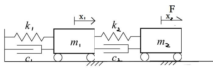
上図のような連成振動を考える。状態方程式を立式する。
m1:質量[kg]
k1:ばね定数[N/m]
c1:粘性減衰係数[N・s/m]
m2:質量[kg]
k2:ばね定数[N/m]
c2:粘性減衰係数[N・s/m]
f:力[N]
とおくと、
上記の運動方程式は、
m_{1}\ddot{x}_{1}+c_{1}\dot{x}_{1}+k_{1}x_{1}-c_{2}(\dot x_{2}-\dot x_{1})-k_{2}(x_{2}-x_{1})=0 \\
m_{2}\ddot{x}_{2}+c_{2}(\dot x_{2}-\dot x_{1})+k_{2}(x_{2}-x_{1})= +f \\
m_{1}\ddot{x}_{1}=-(c_{1}+c_{2})\dot{x}_{1}-(k_{1}+k_{2})x_{1}+c_{2}\dot x_{2}+k_{2}x_{2} \\
m_{2}\ddot{x}_{2}=c_{2}\dot x_{1}+k_{2}x_{1} -c_{2}\dot x_{2}-k_{2}x_{2} +f\\
\begin{bmatrix}
\dot{x}_{1} \\
\ddot{x}_{1} \\
\dot{x}_{2} \\
\ddot{x}_{2} \\
\end{bmatrix}
 =

\begin{bmatrix}
0 & 1 & 0& 0\\
\ -\frac{k_{1}+k_{2}}{m_{1}} & -\frac{c_{1}+c_{2}}{m_{1}} & \frac{k_{2}}{m_{1}} & \frac{c_{2}}{m_{1}}\\
0 & 0 & 0& 1\\
\ \frac{k_{2}}{m_{2}} & \frac{c_{2}}{m_{2}} & -\frac{k_{2}}{m_{2}} & -\frac{c_{2}}{m_{2}}\\
\end{bmatrix}

\begin{bmatrix}
{x}_{1} \\
\dot{x}_{1} \\
{x}_{2} \\
\dot{x}_{2} \\
\end{bmatrix}

+
\begin{bmatrix}
0 \\
0 \\
0 \\
1/m_{2} \\
\end{bmatrix}
f
出力方程式を、m2質点の位置x2を観測する方程式とすると、
y=
\begin{bmatrix}
0 & 0 & 1 & 0
\end{bmatrix}
\begin{bmatrix}
{x}_{1} \\
\dot{x}_{1} \\
{x}_{2} \\
\dot{x}_{2} \\
\end{bmatrix}
となる。
これを状態方程式
\dot{x}(t)=Ax(t)+Bu(t) \\
y(t)=Cx(t)+Du(t)
に当てはめると
A=
\begin{bmatrix}
0 & 1 & 0& 0\\
\ -\frac{k_{1}+k_{2}}{m_{1}} & -\frac{c_{1}+c_{2}}{m_{1}} & \frac{k_{2}}{m_{1}} & \frac{c_{2}}{m_{1}}\\
0 & 0 & 0& 1\\
\ \frac{k_{2}}{m_{2}} & \frac{c_{2}}{m_{2}} & -\frac{k_{2}}{m_{2}} & -\frac{c_{2}}{m_{2}}\\
\end{bmatrix}
,
B=
\begin{bmatrix}
0 \\
0 \\
0 \\
1/m_{2} \\
\end{bmatrix}
,
C=
\begin{bmatrix}
0 & 0 & 1 & 0
\end{bmatrix}
,
D=[0]
とする。
これをPythonControlに入力して、伝達関数を求める。
dual_degree_of_freedom_system.py
# !/usr/bin/env python
from control.matlab import *
from matplotlib import pyplot as plt
def main():
k1=3.0
m1=0.1
c1=0.01
k2=3.0
m2=0.1
c2=0.01
A = [[0., 1,0,0], [-(k1+k2)/m1, -(c1+c2)/m1,k2/m1,c2/m1],[0., 0,0,1],
[-k2/m2,c2/m2,-k2/m2,-c2/m2] ]
B = [[0.], [0.], [0.], [1./m2]]
C = [[0,0,1., 0.0]]
D = [[0.]]
sys1 = ss2tf(A, B, C, D)
print sys1
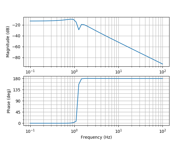
mag, phase, omega = bode(sys1)
plt.show()
if __name__ == "__main__":
main()
$ ./dual_degree_of_freedom_system.py

          10 s^2 + 2 s + 600
--------------------------------------
s^4 + 0.3 s^3 + 90.01 s^2 + 12 s + 2700