更新履歴

(2016/09/25)思いっきりプログラムが間違ってたのでソースコードと実験結果を修正

はじめに

　最小二乗法とかで観測データにモデルフィッティングしたいときに、誤差の大きい観測データに対しては重みを小さくするような重み付き最小二乗法のひとつにM推定というテクニックがあるようです。
　さらに、M推定の中に、TukeyのBiweight推定（重みの設定の仕方がTukeyのBiweight型であるM推定）というテクニックがあるようです。

有名なテクニックのようで、既にネット上でも多くの解説記事がありますが、お手軽に試せるコードを見つけられなかったので、試しに2次元の直線を推定するプログラムを書いてみました。

問題設定

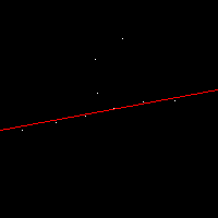
2次元の画像上の白い点群に対して直線をフィッティングする。先に結果を載せてしまいますが、以下の図の白い点に対して赤い線を推定する問題です。

処理の流れ

重み係数を初期化
重み付き最小二乗
重み係数を更新
1.～3.をT回繰り返す

以降に記述するプログラムでは、繰り返し回数T=3としました。また、繰り返し処理を終了する判定基準には、他にも残差を見たり色々あるようです。

式

直線の式

y = ax + b

重み付き最小二乗の式

\begin{pmatrix}
\sum_i w_i x_i^2 & \sum_i w_i x_i \\
\sum_i w_i x_i   & \sum_i w_i 
\end{pmatrix}
\begin{pmatrix}
a \\
b
\end{pmatrix}
=
\begin{pmatrix}
\sum_i w_i x_i y_i \\
\sum_i w_i y_i   
\end{pmatrix}

x、y はそれぞれサンプル点の座標値です。wは重み係数です。a、bは直線の方程式のパラメーターで傾きとy切片です。このaとbが推定されます。

重み係数の更新式

{w_i = \left\{
\begin{array}{ll}
\bigl\{ 1 - (\frac{d_i}{c})^2 \bigr\} ^2 & (d_i \leq c)\\
0 & (d_i \gt c)
\end{array}
\right.
}

ここで、

d_i = |y_i - (a x_i + b)|

は、推定直線とサンプル点の差です。cはサンプル点の誤差に関する閾値です。外れ点の影響を無くす効果があると思います。
※d≦c のときの重み係数の更新式に2乗が2つありますが、最初、外側の2乗を忘れてプログラムを実装してしまいました。しかし、それでもうまく推定できました。更新式の背景にある理論をしっかり理解していないので、違いが良く分かっていません。

ソースコードとデータ

ソースはc++とpythonそれぞれで書いてみました。

入力画像

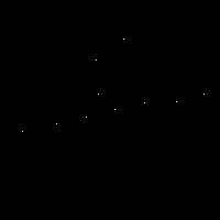
入力画像（pts.png）は以下です。

ソース(c++)

#include "opencv2\opencv.hpp"

using namespace cv;

int main(int argc, char* argv[])
{
    // 点情報入力
    const Mat1b im = imread("pts.png", 0);

    vector<Point> pts;
    cv::findNonZero(im, pts);

    // 重み係数の初期化
    vector<double> weight(pts.size(), 1.0);

    const int    T = 3; // 最大繰り返し回数
    const double c = 20;
    int t = 0;

    while (t < T) {

        // 重み付き最小二乗
        Mat1d A = Mat1d::zeros(2, 2);
        Mat1d b = Mat1d::zeros(2, 1);
        for (size_t p = 0; p < pts.size(); ++p){
            double w = weight[p];
            A(0, 0) += w * pts[p].x * pts[p].x;
            A(1, 0) += w * pts[p].x;
            A(1, 1) += w;
            b(0, 0) += w * pts[p].x * pts[p].y;
            b(1, 0) += w * pts[p].y;
        }
        A(0, 1) = A(1, 0);

        Mat1d x;
        cv::solve(A, b, x);

        // 推定直線を描画
        Point start(0, int(x(1, 0) + 0.5));
        Point end(im.cols - 1, int(x(0, 0) * (im.cols - 1) + x(1, 0) + 0.5));
        Mat plot_im = imread("pts.png");
        cv::line(plot_im, start, end, Scalar(0, 0, 255));
        imwrite(format("plot_itr%02d.png", t), plot_im);

        // 重みの更新      
        for (size_t p = 0; p < pts.size(); ++p){
            double dif = fabs( pts[p].y - (x(0, 0) * pts[p].x + x(1, 0))); // dif = |y - (ax + b)|
            weight[p] = (dif > c) ? 0.0 : pow(1.0 - (dif / c) * (dif / c), 2);
        }

        ++t;
    }
    return 0;
}

ソース(python)

import numpy as np
import cv2

im = cv2.imread('pts.png', 0)

y, x = np.where(im)
weight = np.ones((len(x)))

T = 3
c = 20.0

t = 0
while t < T:
    A = np.zeros((2,2))
    b = np.zeros((2))
    A[0,0] = np.sum(weight * x * x)
    A[1,0] = np.sum(weight * x)
    A[0,1] = A[1,0]
    A[1,1] = np.sum(weight)
    b[0]   = np.sum(weight * x * y)
    b[1]   = np.sum(weight * y)

    coef = np.linalg.solve(A, b)

    # Plot the estimated line
    start_x = 0
    start_y = int(coef[0] * start_x + coef[1] + 0.5)# y = ax + b
    end_x   = im.shape[1] - 1
    end_y   = int(coef[0] * end_x + coef[1] + 0.5)# y = ax + b

    plot_im = cv2.imread('pts.png')    
    cv2.line(plot_im,(start_x, start_y),(end_x, end_y),(0,0,255),1)
    cv2.imwrite('plot_itr{}.png'.format(t), plot_im)

    # Update weights
    dif                     = np.abs(y - (coef[0] * x + coef[1]))
    outlier_indices         = np.where(dif > c)
    inlier_indices          = np.where(dif <= c)
    weight[outlier_indices] = 0.0
    weight[inlier_indices]  = (1.0 - (dif[inlier_indices] / c) ** 2) ** 2

    t += 1

実行すると以下のようなフィッティング結果画像が出力されます。

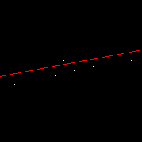
繰り返し処理の1回目の推定結果

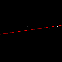
繰り返し処理の2回目の推定結果

繰り返し処理の3回目の推定結果

なんかうまくいっているように見えますね？
というか、うまくいくようにc（重み係数を更新するときに使うパラメーター）を設定したからですが。。。cを小さい値にしたら、重み係数が更新時に全部ゼロになりました。TukeyのBiweight推定法について、根本的に勘違いしている可能性があるかも？

TukeyのBiweight推定法を使って画像中の点群から直線推定