最近 Rust が流行っていますね。ご多分に漏れず私も始めてみたのですが、Hello, World! をクリアした後、何を作るとRustっぽいのか悩みました。GUIが得意な言語でもないですし。
そこで今回は、Numpyで書いた差動二輪型自律移動ロボットのシミュレータを、Rustで再実装してみました。自律移動ロボットは、自己位置推定や局所経路探索のために行列演算を高速に繰り返すので、演算性能に優れたRustの題材としては良さげな気がします。ソースコードは robot_simulator_rust です。ではいってみよう！

シミュレートする状況

あるルールに従って移動するターゲットを、差動二輪型自律移動ロボットが追いかけます。ただしロボットはタイヤのスリップや路面の細かな段差のために、指定した入力どおりには移動できず、移動後のロボットの姿勢（$x$座標、$y$座標、及びロボットの向き）には僅かな誤差が含まれるものとします。

出典：東北学院大学工学部機械知能工学科 RDE 熊谷正朗車輪移動ロボット http://www.mech.tohoku-gakuin.ac.jp/rde/contents/course/robotics/wheelrobot.html

またロボットには360度カメラが搭載されており、外部に設置されているマーカーまでの距離と方向を、マーカーの正確な$x$座標と$y$座標と対応付けて観測することができます。ただしロボットが観測したマーカーまでの距離と方向には、やはり僅かな誤差が含まれてしまうものとします。

このような状況下で、与えられたルールに従ってロボットが自律移動できるように、拡張カルマンフィルタを用いた自己位置推定と Dynamic Window Approachもどきを用いた局所経路計画を実装します。

なお今回は計算を簡単にするために、各誤差は特定の傾向を持たない白色ガウス雑音と仮定しています。

シミュレーション結果

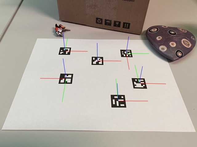
以下に３つのルールに対してシミュレートした結果を図示します（図中に描かれる線などの意味は、次表を参考）。

線や四角形	意味
黒のマーク	指定されたルールに従って移動するターゲット
黒の線	理想の軌跡
灰色の正方形	観測されるマーカー
緑の線	ロボットが観測したマーカーの方向と距離
赤のマーク	ロボットが推定した自身の姿勢（位置と向き）
赤の線	ロボットが推定した自己位置の軌跡
青の線	実際にロボットが移動した軌跡（ロボット自身は観測しえない）

円と線分で構成されたマークは、円の中心がロボットの位置、中心から外周に向かう線分がロボットの向きを表しています。

これらのルールは、Agent traitを実装した構造体のget_idealメソッドにて定義していますので、構造体を作成し新たなルールを自分で追加することもできます。

src/agent/circular_agent.rs

impl Agent for CircularAgent {
  /// Get the ideal pose that moves on the circumference at a constant angular velocity
  ///
  /// ## Arguments
  /// * `_` - current pose of robot which is defined as nalgebra::Vector3::new(x, y, theta)
  ///     *  Since the current pose is not used in this function, the argument name is defind as `_`
  /// * `t` - elapsed time (sec) from the start of this simulation
  ///
  /// ## Returns
  /// ideal pose of robot which is defined as nalgebra::Vector3::new(x, y, theta)
  fn get_ideal(&self, _: &na::Vector3<f64>, t: f64) ->  na::Vector3<f64> {
    let angle = INPUT_OMEGA * t;
    let x = angle.cos();
    let y = angle.sin();
    let theta = utils::normalize_angle(angle + PI / 2.0);

    na::Vector3::new(x, y, theta)
  }

ルール１：円を描く

一定の角速度で円を描いて移動するターゲットを追いかけます。

ルール2：正方形を描く

一定の距離進んだ後に反時計回りで90度回転、を繰り返すことで正方形の外周上を移動するターゲットを追いかけます。

本来の差動二輪型自律移動ロボットであれば、その場で旋回（超信地旋回）する際にここまで左右にズレたりしませんが、それはシミュレータの設定が甘いということで・・・

ルール3：waypointを追いかける

ロボットが指定された姿勢（位置と向き）に大体一致すると、次の姿勢へと瞬間移動するターゲット（waypoint）を追いかけます。

環境

	バージョン
Rust	1.51.0
OS	macOS Big Sur 11.5.1

シミュレータの可視化部分をRustで書くのは大変そうだったので、 Python 3.9上の別プロセスで動作する plotter を実装しています。シミュレータ本体のRust部分とは ZeroMQ で通信しています。

動作方法

plotterの起動

pyenvを用い、tck-tkをincludeしてpython 3.9をインストール

$ brew install tcl-tk
$ env \
  PATH="$(brew --prefix tcl-tk)/bin:$PATH" \
  LDFLAGS="-L$(brew --prefix tcl-tk)/lib" \
  CPPFLAGS="-I$(brew --prefix tcl-tk)/include" \
  PKG_CONFIG_PATH="$(brew --prefix tcl-tk)/lib/pkgconfig" \
  CFLAGS="-I$(brew --prefix tcl-tk)/include" \
  PYTHON_CONFIGURE_OPTS="--with-tcltk-includes='-I$(brew --prefix tcl-tk)/include' --with-tcltk-libs='-L$(brew --prefix tcl-tk)/lib -ltcl8.6 -ltk8.6'" \
  pyenv install 3.9.5

リポジトリをclone

$ git clone https://github.com/nmatsui/robot_simulator.git
$ cd robot_simulator/

pipenvを用いてライブラリをインストール
```
pipenv install
```
plotterを起動
```
$ pipenv run plotter
```

シミュレータの起動

リポジトリをclone

$ git clone https://github.com/nmatsui/robot_simulator_rust.git
$ cd robot_simulator_rust/

releaseバイナリをビルド
```
$ cargo build --release
```
シミュレータを起動（引数は circular, square, waypoints のどれか）
```
$ ./target/release/robot_simulator_rust circular
```

シミュレータの詳細

ロボットの運動状態のモデル化

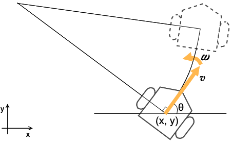
ある地点 $(x, y)$ で $x$軸からの角度 $\theta$ を向いたロボットに対して、ある入力 $u$ （並進速度 $v$ [m/s] 角速度 $\omega$ [rad/s]）を与えると、下の図のようにプログラムの1回分の計算サイクル後にロボットは次の姿勢まで移動します。この間、 $v$ と $\omega$ は変化しません。

この運動を、以下のようにモデル化します。

\hat{x}_{k|k-1} = f(\hat{x}_{k-1|k-1},u_{k}) + w_{k}

ここで $\hat{x}_{k-1|k-1}$は移動を開始する前のロボットの姿勢 $(x_{k-1}, y_{k-1}, \theta_{k-1})$ 、 $u_{k}$ はロボットを移動させるために与えた入力 $(v, \omega)$ であり、 $f$ は $\hat{x}$ と $u$ の何らかの非線形な関数、 $w_{k}$ はロボットが移動すると誤差が含まれてしまうことを表す共分散行列が $Q$ で平均が0の白色ガウス雑音です。これらを用いて、移動後のロボットの姿勢 $\hat{x}_{k|k-1}$を算出することができます。

ここで $f$ を立式したいのですが、移動を開始する前のロボットの姿勢 $\hat{x}_{k-1|k-1}$ に、入力された速度 $u_{k}$ をプログラムの計算サイクル $\varDelta{t}$ で積分したものを加えれば、次の姿勢 $\hat{x}_{k|k-1}$ になります。この関係から $f$ を立式できますが、真面目に積分するのがちょっと面倒です。そこで今回は プログラムの計算サイクル $\varDelta{t}$ における回転角 $\varDelta{\theta}$は十分に小さい と仮定して、本来円弧を描くロボットの移動軌跡を次のように直線で近似して $f$ を立式します。

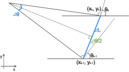
この図より、 $\hat{x}_{k|k-1}$ と $\hat{x}_{k-1|k-1}$ の関係を次のように表すことができます。

x_{k} = x_{k-1}+\varDelta{L}\cos(\theta_{k-1}+\frac{1}{2}\varDelta{\theta})

y_{k} = y_{k-1}+\varDelta{L}\sin(\theta_{k-1}+\frac{1}{2}\varDelta{\theta})

\theta_{k} = \theta_{k-1}+\varDelta{\theta}

また $\varDelta{L}$ と $\varDelta{\theta}$ は、 $\varDelta{t}$ と $u$ を用いて次のように書けます。

\varDelta{L} = \it{v}\varDelta{t}

\varDelta{\theta} = \it{\omega}\varDelta{t}

これらから、 $f$ は $\hat{x}_{k-1|k-1}$ と $u$ を用いて次のように表すことができます。

\it_{f}
=
\left(
  \begin{array}{c}x_{k-1}\\y_{k-1}\\\theta_{k-1}\end{array}
\right)
+
\left(
  \begin{array}{cc}\cos(\theta_{k-1}+\frac{1}{2}\omega\varDelta{t})\varDelta{t}&0\\\sin(\theta_{k-1}+\frac{1}{2}\omega\varDelta{t})\varDelta{t}&0\\0&\varDelta{t}\end{array}
\right)
\left(
  \begin{array}{c}\it{v}\\\it{\omega}\end{array}
\right)

このモデル（状態方程式）を実装したのが、models::robotモジュールのideal_move関数です。色々とややこしいことを考えてたわりに、関数はシンプルです。

src/models/robot.rs

/// Calculate the state equation of a simulated robot
///
/// ## Arguments
/// * `current` - the current pose of the simulated robot(x, y, theta)
/// * `input` - the input vector(linear velocity, angular velocity)
/// * `delta` - time delta to next tick
///
/// ## Returns
/// The pose(x, y, theta) of the simulated robot at the next tick
pub fn ideal_move(current: &na::Vector3<f64>, input: &na::Vector2<f64>, delta: f64) -> na::Vector3<f64> {
  let a = current[2] + input[1] * delta / 2.0;
  let m = na::Matrix3x2::new(a.cos() * delta, 0.0,
                             a.sin() * delta, 0.0,
                             0.0,             delta);
  let mut next = current + m * input;
  next[2] = utils::normalize_angle(next[2]);
  next
}

カメラによるマーカー観測のモデル化

ロボットに据え付けられたカメラでマーカーを観測すると、カメラの視界内にマーカーが写ります。ここで使うマーカーは、例えばArUcoマーカーのような、マーカーの見え方によってカメラからマーカーまでの距離とカメラ座標系におけるマーカーの位置と方向を推定できるものとします。

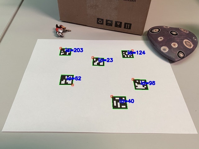
出典： OpenCV 4.5.2 Detection of ArUco Markers 　https://docs.opencv.org/4.5.2/d5/dae/tutorial_aruco_detection.html

ただし実際のカメラとArUcoマーカーでは３次元空間内でのマーカー姿勢を算出しますが、今回考えているロボットは $(x, y)$ の２次元平面上を移動します。そこでマーカーは $(x, y)$ 平面上に存在し、カメラはその平面上のマーカーまでの距離 $d_{m}$ [m] と、カメラ正面からの角度 $\phi_{m}$ [rad] が観測できるものとします。また、マーカーのIDとロボット座標系における位置を対応付けておき、観測したマーカーの絶対的な位置 $(x_{m}, y_{m})$ が得られるものとします。

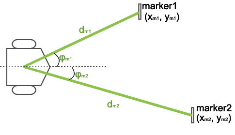
このマーカーの観測を、以下のようにモデル化します。

z_{k} = h(\hat{x}_{k|k-1}) + v_{k}

ここで $\hat{x}_{k|k-1}$ はマーカーを観測した時点でのロボットの姿勢 $(x_{k-1}, y_{k-1}, \theta_{k-1})$ 、 $z_{k}$ はロボットが観測したマーカーの情報 $(d_{m}, \phi_{m})$ であり、 $h$ は $\hat{x}$ に関する非線形な関数、 $v_{k}$ はロボット観測したマーカーの位置と角度には誤差が含まれてしまうことを表す共分散行列が $R$ で平均が0の白色ガウス雑音です。

$h$ はシンプルに、幾何学的な関係から立式することができます。

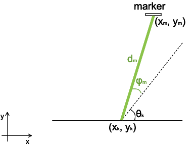
d_{m} = \sqrt{(x_{m}-x_{k})^2 + (y_{m}-y_{k})^2}

\phi_{m} = tan^{-1}\left(\frac{y_{m}-y_{k}}{x_{m}-x_{k}}\right) - \theta_{k}

このモデル（観測方程式）を実装したのが、 models::camera モジュールの observe 関数です。そのまんまですね。

src/models/camera.rs

/// Calculate the observation equation of a camera
///
/// ## Arguments
/// * `landmark` - the observed landmark
/// * `current` - the current pose of the simulated robot(x, y, theta)
///
/// ## Returns
/// An observed vector(distance, angle)
pub fn observe(landmark: &Point, current: &na::Vector3<f64>) -> na::Vector2<f64> {
  let dist = (na::Vector2::new(landmark.x, landmark.y) - current.fixed_rows::<2>(0)).norm_squared().sqrt();
  let angle = (landmark.y - current[1]).atan2(landmark.x - current[0]) - current[2];
  na::Vector2::new(dist, angle)
}

※ NargeblraのMatrix::norm_squaredは、２ベクトル間のL2ノルムの二乗を求めるメソッドです。計算速度を向上させるためにわざわざ二乗したままの結果を返すのに、後から平方してダイナシにしてしまうという（笑

拡張カルマンフィルタを用いた自己位置推定

上述したモデルを用いて、ロボットの自己位置を推定します。

予測ステップ

$f$ は非線形のため、線形近似するためにヤコビアン $F_{k-1}$ を計算しておきます（calc_f 関数）。

F_{k-1}
=
\left.\frac{\partial f(\hat{x},u)}{\partial \hat{x}}\right|_{x=\hat{x}_{k-1|k-1},u=u_{k}}
=
\left(
  \begin{array}{ccc}
    \frac{\partial x_{k}}{\partial x_{k-1}}&\frac{\partial x_{k}}{\partial y_{k-1}}&\frac{\partial x_{k}}{\partial \theta_{k-1}}\\
    \frac{\partial y_{k}}{\partial x_{k-1}}&\frac{\partial y_{k}}{\partial y_{k-1}}&\frac{\partial y_{k}}{\partial \theta_{k-1}}\\
    \frac{\partial \theta_{k}}{\partial x_{k-1}}&\frac{\partial \theta_{k}}{\partial y_{k-1}}&\frac{\partial \theta_{k}}{\partial \theta_{k-1}}
  \end{array}
\right)
=
\left(
  \begin{array}{ccc}
    1&0&-\it{v}\varDelta{t}\sin(\theta_{k-1}+\frac{1}{2}\omega\varDelta{t})\\
    0&1&\it{v}\varDelta{t}\cos(\theta_{k-1}+\frac{1}{2}\omega\varDelta{t})\\
    0&0&1
  \end{array}
\right)

src/models/robot.rs

/// Calculate the jacobian of the state equation
///
/// ## Arguments
/// * `current` - the current pose of the simulated robot(x, y, theta)
/// * `input` - the input vector(linear velocity, angular velocity)
/// * `delta` - time delta to next tick
///
/// ## Returns
/// The jacobian of the state equation
pub fn calc_f(current: &na::Vector3<f64>, input: &na::Vector2<f64>, delta: f64) -> na::Matrix3<f64> {
  let a = current[2] + input[1] * delta / 2.0;

  na::Matrix3::new(1.0, 0.0, -1.0 * a.sin() * delta * input[0],
                   0.0, 1.0,  1.0 * a.cos() * delta * input[0],
                   0.0, 0.0,  1.0)
}

まずは $f$ を用いて、事前状態を計算します。

\hat{x}_{k|k-1} = f(\hat{x}_{k-1|k-1},u_{k}) = \left(
  \begin{array}{c}x_{k-1}\\y_{k-1}\\\theta_{k-1}\end{array}
\right)
+
\left(
  \begin{array}{cc}\cos(\theta_{k-1}+\frac{1}{2}\omega\varDelta{t})\varDelta{t}&0\\\sin(\theta_{k-1}+\frac{1}{2}\omega\varDelta{t})\varDelta{t}&0\\0&\varDelta{t}\end{array}
\right)
\left(
  \begin{array}{c}\it{v}\\\it{\omega}\end{array}
\right)

次に次式で事前誤差共分散行列 $P_{k|k-1}$ を得ます。ここで $Q$ は $w_{k}$ の共分散行列です。今回は簡単にするため、 $Q$ は時間変化せず一定としています。

P_{k|k-1} = F_{k-1}P_{k-1|k-1}F_{k-1}^{T} + Q

rustで実装するとこんな感じです（filters::kalman_filter::EKF構造体のpredict関連関数）。言われたとおりに実装しているだけですね。

src/filters/kalman_filter.rs

  /// **\[private\]** Calculate the "predict step"
  ///
  /// ## Arguments
  /// * `xhat` - the current estimated pose(x, y, theta)
  /// * `p` - the current covariance matrix
  /// * `q` - the covariance matrix of process noise
  /// * `input` - the current input vector(linear velocity, angular velocity)
  /// * `delta` - time delta
  ///
  /// ## Returns
  /// Tuple of (predicted pose(x, y, theta), predicted covariance matrix)
  fn predict(xhat: &na::Vector3<f64>, p: &na::Matrix3<f64>, q: &na::Matrix3<f64>, input: &na::Vector2<f64>, delta: f64)
    -> (na::Vector3<f64>, na::Matrix3<f64>) {
    let a_priori_x = robot::ideal_move(xhat, input, delta);
    let f = robot::calc_f(xhat, input, delta);
    let a_priori_p = f * p * f.transpose() + q;
    (a_priori_x, a_priori_p)
  }

更新ステップ

同様に $h$ も非線形のため、線形近似するためにヤコビアン $H_{k}$ を計算しておきます（calc_h 関数）。

H_{k}
=
\left.\frac{\partial h(\hat{x})}{\partial \hat{x}}\right|_{x=\hat{x}_{k|k-1}}
=
\left(
  \begin{array}{ccc}
    \frac{\partial d_{m}}{\partial x_{k}}&\frac{\partial d_{m}}{\partial y_{k-1}}&\frac{\partial d_{m}}{\partial \theta_{k-1}}\\
    \frac{\partial \phi_{m}}{\partial x_{k-1}}&\frac{\partial \phi_{m}}{\partial y_{k-1}}&\frac{\partial \phi_{m}}{\partial \theta_{k-1}}\\
  \end{array}
\right)
=
\left(
  \begin{array}{ccc}
    -\frac{x_{m}-x_{k}}{\sqrt{(x_{m}-x_{k})^2+(y_{m}-y_{k})^2}}&-\frac{y_{m}-y_{k}}{\sqrt{(x_{m}-x_{k})^2+(y_{m}-y_{k})^2}}&0\\
    \frac{y_{m}-y_{k}}{(x_{m}-x_{k})^2+(y_{m}-y_{k})^2}&-\frac{x_{m}-x_{k}}{(x_{m}-x_{k})^2+(y_{m}-y_{k})^2}&-1
  \end{array}
\right)

src/models/camera.rs

/// Calculate the jacobian of the observation equation
///
/// ## Arguments
/// * `landmark` - the observed landmark
/// * `current` - the current pose of the simulated robot(x, y, theta)
///
/// ## Returns
/// The jacobian of the observation equation
pub fn calc_h(landmark: &Point, current: &na::Vector3<f64>) -> na::Matrix2x3<f64> {
  let q = (landmark.x - current[0]).powf(2.0) + (landmark.y - current[1]).powf(2.0);

  na::Matrix2x3::new((current[0] - landmark.x)/q.sqrt(), (current[1] - landmark.y)/q.sqrt(),  0.0,
                     (landmark.y - current[1])/q,        (current[0] - landmark.x)/q,        -1.0)
}

$h$ を用いて、実際に観測したデータと予測した位置から観測したら得られるはずのデータとの誤差（観測残差）を計算します。

\hat{y}_{k} = z_{k} - h(\hat{x}_{k|k-1})
=
\left(
  \begin{array}{c}d_{m}\\\phi_{m}\end{array}
\right)
-
\left(
  \begin{array}{c}\sqrt{(x_{m}-x_{k})^2 + (y_{m}-y_{k})^2}\\tan^{-1}\left(\frac{y_{m}-y_{k}}{x_{m}-x_{k}}\right) - \theta_{k}\end{array}
\right)

$H_{k}$ と事前誤差共分散行列 $P_{k|k-1}$ を用いて観測残差の共分散を計算し、カルマンゲイン $K_{k}$ を得ます。ここで $R$ は $v_{k}$ の共分散行列ですが、 $Q_{k}$ と同様に時間変化せず一定としています。

S_{k} = H_{k}P_{k|k-1}H_{k}^{T} + R

K_{k} = P_{k|k-1}H_{k}^{T}S_{k}^{-1}

カルマンゲイン $K_{k}$ と観測残差 $\hat{y}_{k}$ を用いて、予測した状態 $\hat{x}_{k|k-1}$ を更新します。

\hat{x}_{k|k} = \hat{x}_{k|k-1} + K_{k}\hat{y}_{k}

最後に誤差共分散行列を更新し、次回のステップに備えます。

P_{k|k} = (I-K_{k}H_{k})P_{k|k-1}

rustで実装するとこんな感じです（filters::kalman_filter::EKF 構造体の update 関連関数）。

src/filters/kalman_filter.rs

  /// **\[private\]** Calculate the "update step"
  ///
  /// ## Arguments
  /// * `r` - the covariance matrix of observation noise
  /// * `a_priori_x` - the predicted pose(x, y, theta)
  /// * `a_priori_p` - the predicted covariance matrix
  /// * `observed` - observed landmark
  ///
  /// ## Returns
  /// * Tuple of (estimated pose(x, y, theta), covariance matrix, kalman gain)
  fn update(r: &na::Matrix2<f64>, a_priori_x: &na::Vector3<f64>, a_priori_p: &na::Matrix3<f64>, observed: &Observed)
    -> (na::Vector3<f64>, na::Matrix3<f64>, na::Matrix3x2<f64>) {
    let yhat = na::Vector2::new(observed.distance, observed.angle) - camera::observe(&observed.landmark, a_priori_x);
    let h = camera::calc_h(&observed.landmark, a_priori_x);
    let s = h * a_priori_p * h.transpose() + r;
    let k = a_priori_p * h.transpose() * s.try_inverse().unwrap();
    let xhat = a_priori_x + k * yhat;
    let p = (na::Matrix3::identity() - k * h) * a_priori_p;
    (xhat, p, k)
  }
}

観測したマーカーの数だけ更新ステップを繰り返すことで、拡張カルマンフィルタの１サイクルが完了します。このサイクルを延々と繰り返すことで、ロボットの現在位置を逐次的に推定することが可能となります。

src/filters/kalman_filter.rs

  pub fn step(&mut self) -> ... {
...
    let (mut xhat, mut p) = EKF::predict(&self.xhat, &self.p, &self.q, &input, delta);
    let mut k: na::Matrix3x2<f64> = na::Matrix3x2::zeros();
    for observed in self.agent.noisy_observe() {
      let (updated_xhat, updated_p, updated_k) = EKF::update(&self.r, &xhat, &p, observed);
      xhat = updated_xhat;
      p = updated_p;
      k = updated_k;
    }

    self.xhat = xhat;
    self.p = p;
    self.t = t;
...
  }

Dynamic Window Approachもどきを用いた局所経路計画

拡張カルマンフィルタを用いて自己位置が推定できたので、次はターゲットを追いかけるために最適な入力を計算します。ロボットの運動モデルを元に最適な入力を計算するアルゴリズムは種々提案されていますが、今回は実装がシンプルなDynamic Window Approachもどきを実装します（障害物回避を実装していないので、もどき なのです）。

サンプリングする速度空間（Dynamic Window）の探索

まずはロボットが実際に動作可能な速度の範囲を求めます。ロボットのスペック（最大並進加速度・最大角加速度、最大並進速度・最小並進速度、最大角速度・最小角速度）と現在のロボットの並進速度と角速度から、次の計算サイクルで実際に動作可能な並進速度・角速度の最小値と最大値を計算します。

ここで求めた実現可能な並進速度・角速度の範囲を、事前に決めておいたサンプリングレートで区切り、次の計算サイクルで実行可能な並進速度・角速度をリスト化します。

本来のDWAであれば、障害物に近づきすぎる（あるいは衝突する）速度の組み合わせは取り除くのですが、今回のロボットは障害物を検知するセンサを積んでいない（という設定）のため、この障害物回避処理は割愛しています。