はじめに
学部学生の実験の解析手順書とサンプルプログラムを書くために、色々なプログラムを使って、適当なデータを最小二乗法でフィットする方法を調べてみたので、そのメモを残す。
最小二乗法を使うという点で、原理は同じなので同じ結果を出してもらわないと困るんだけど、残念ながらプログラムによって答えが違う、というところまでは以前から知っていたんだけど、最近その原因と対処法が書いてあるテキストを見つけたので自分のために整理してみることにした。きっかけとなったテキストというのは、これ。
Peter Young, "Everything you wanted to know about Data Analysis and Fitting but were afraid to ask"
どうやら、大学の講義資料らしい。ここで、GnuplotとPythonのscipy.optimize.curve_fitは、データに誤差がある場合に、結果のパラメータに付くエラーの数値が間違っているので修正する必要がある、とある。
Gnuplotの場合は、端的にはこのように修正が必要。
to get correct error bars on fit parameters from gnuplot when there are error bars on the points, you have to divide gnuplot’s asymptotic standard errors by the square root of the chi-squared per degree of freedom (which gnuplot calls FIT STDFIT and, fortunately, computes correctly).
pythonのscipy.optimizeの場合は複雑で、curve_fitは修正の必要があるが、leastsqは修正の必要がない。
I recently learned that error bars on fit parameters given by the routine curve_fit of python also have to be corrected in the same way. This is shown in two of the python scripts in appendix H. Curiously, a different python fitting routine, leastsq, gives the error bars correctly.
なんでこれに誰も気づいていないのか疑問だ、と書いてある。
It is curious that I found no hits on this topic when Googling the internet.
サンプルデータ
こんなデータセットを用意した。(x,y,ey)のセットが20個。これを直線でフィットすることにする。テキストファイルdata.txtという名前で保存しておくことにする。
0.0e+00 -4.569987720595017344e-01 1.526828747143463172e+00
1.0e+00 -7.106162255269843353e-01 1.402885069270964458e+00
2.0e+00 1.105159634902675325e+00 1.735638554786020915e+00
3.0e+00 -1.939878950652441869e+00 1.011014634823069747e+00
4.0e+00 3.609690931525689983e+00 1.139915698020605550e+00
5.0e+00 8.535035219721383015e-01 9.338187791237286817e-01
6.0e+00 4.770810591544029755e+00 1.321364026236713451e+00
7.0e+00 3.323982457761388787e+00 1.703973901689593173e+00
8.0e+00 3.100622722027332578e+00 1.002313080286136637e+00
9.0e+00 4.527766245564444070e+00 9.876090792441625243e-01
1.0e+01 1.990062497396323682e+00 1.355607177365929505e+00
1.1e+01 5.113013340421659336e+00 9.283045349565146598e-01
1.2e+01 4.391676777018354905e+00 1.337677147217683160e+00
1.3e+01 5.388022504497612886e+00 9.392443558621643707e-01
1.4e+01 1.134921361159764075e+01 9.232583484294124565e-01
1.5e+01 6.067025020573844074e+00 1.186258237028150475e+00
1.6e+01 1.052771612360148445e+01 1.200732350014090954e+00
1.7e+01 6.221953870216905713e+00 8.454085761899273743e-01
1.8e+01 9.628358150028700990e+00 1.442970173161927772e+00
1.9e+01 9.493784288063746857e+00 8.196526623903285236e-01
色々なプログラムでのサンプルコード
CERNのROOT
ROOTというのはこれ。
https://root.cern.ch
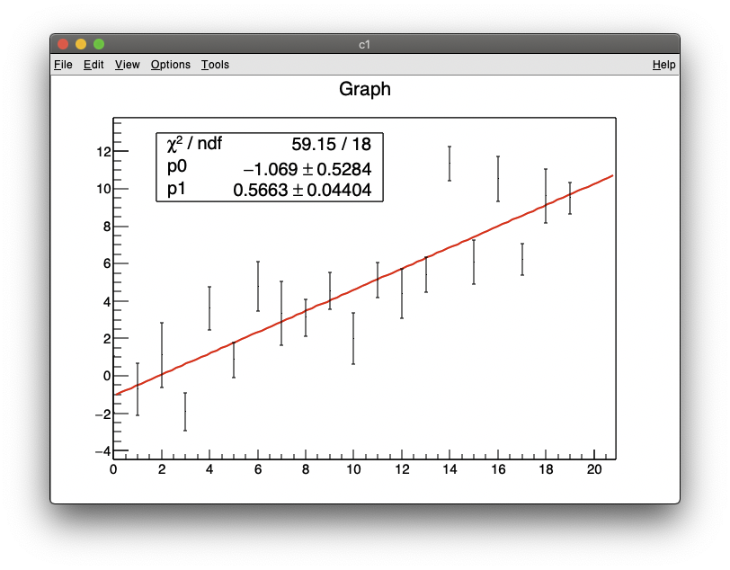
一番コードは短くて済んだ。ROOTの場合は、簡単なものならばフィット関数を定義しなくても用意されてるからね。
{
  TGraphErrors *g = new TGraphErrors("data.txt","%lg %lg %lg");
  g->Fit("pol1");
  g->Draw("ape");
}
結果はこんな感じ。
Gnuplot
Gnuplotも関数でフィットするのは得意なので、必要なコードはとても短い。gnuplotの問題は、デフォルトの出力の見栄えがイマイチすぎることだと思う。
set fit errorvariables

f(x) = p0 + p1*x
fit f(x) "data.txt" u 1:2:3 via p0,p1

plot "data.txt" u 1:2:3 w yerr, f(x)

print "\n ====== ERROR CORRECTED ========"
print "Chi2/NDF = ",FIT_STDFIT**2 * FIT_NDF,"/",FIT_NDF
print "  p0 = ",p0," +- ",p0_err/FIT_STDFIT
print "  p1 = ",p1," +- ",p1_err/FIT_STDFIT

# --------- 以下は図の見栄え調整 --------

set term qt font "Helvetica"
set xrange [-1:20]
set rmargin 5
set tics font ",16"
set key font ",16"
set key left top
set bars fullwidth 0
set style line 1 lc "#0080FF" lw 1 pt 7 ps 1
set style line 2 lc "#FF3333" lw 2 pt 0 ps 1

set label 1 at first 1,11 sprintf("Chi2/ndf = %5.2f / %2d",FIT_STDFIT**2 * FIT_NDF,FIT_NDF) font ",18"
set label 2 at first 1,10 sprintf("p0 = %6.3f +- %7.4f",p0,p0_err/FIT_STDFIT) font ",18"
set label 3 at first 1,9  sprintf("p1 = %6.4f +- %7.5f",p1,p1_err/FIT_STDFIT) font ",18"

plot "data.txt" u 1:2:3 w yerr ls 1,\
     f(x) ls 2
標準出力されるところに書いてある"Asymptotic Standard Error"というのは間違いで、これを修正する必要がある。具体的には、上のコードにあるように、エラーの値をFIT_STDFITという変数で割る。set fit errorvariablesと始めに書いておくと、変数名_errでエラーの数値も拾うことができる。修正するとROOTと同じ値が出てくる。
Final set of parameters            Asymptotic Standard Error
=======================            ==========================
p0              = -1.06859         +/- 0.9578       (89.64%)
p1              = 0.566268         +/- 0.07983      (14.1%)

correlation matrix of the fit parameters:
                p0     p1
p0              1.000
p1             -0.884  1.000

 ====== ERROR CORRECTED ========
Chi2/NDF = 59.1533703771407/18
  p0 = -1.06858871709936 +- 0.528376469987239
  p1 = 0.566267669300731 +- 0.0440357299923021
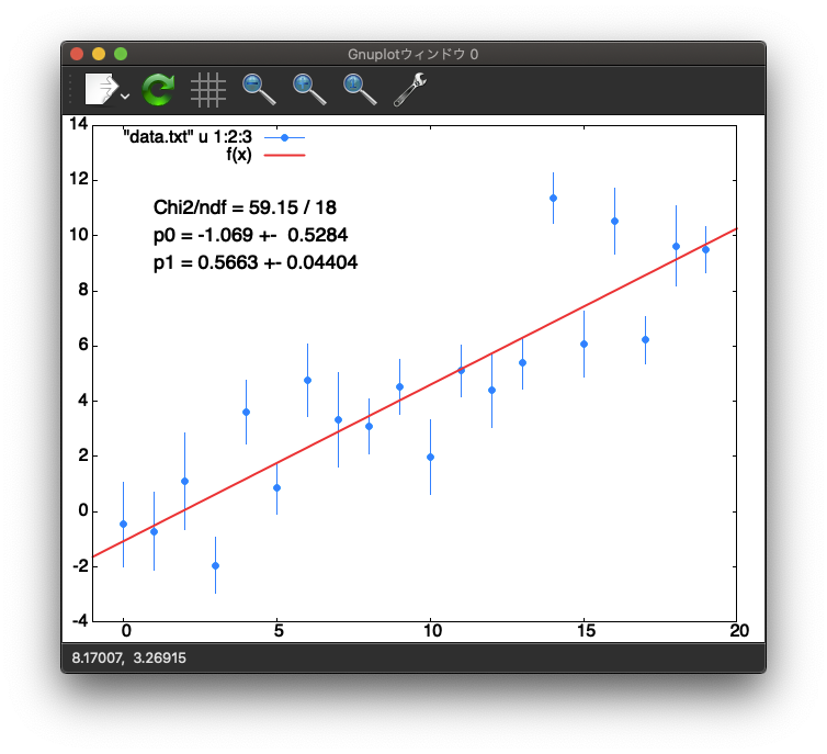
気をつけないとならないのは、このエラーの修正は、データ点に誤差がある場合(fitコマンドでデータを拾うときにusingの後に3つ列を指定するとき)のみ行う必要があること。すべて同じ重みで(=誤差なしのデータを)フィットする場合はこの修正をしてはいけない。
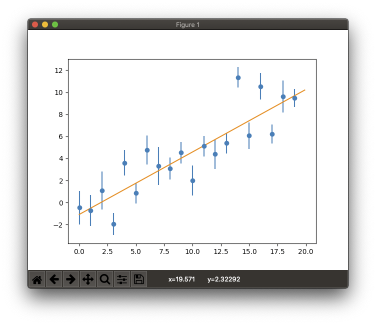
pythonのscipy.optimize.curve_fit
データの読み込みは、numpy.loadtxtを使ったら簡単にできた。
# データを読み込む
import numpy as np

data = np.loadtxt("data.txt")
xx = data.T[0]
yy = data.T[1]
ey = data.T[2]

# フィットする関数ffを定義する
def ff(x,a,b):
    return a + b*x

# フィットして結果を表示する
from scipy.optimize import curve_fit
import math

par, cov = curve_fit(ff,xx,yy,sigma=ey)

chi2 = np.sum(((ff(xx,par[0],par[1])-yy)/ey)**2)
print("chi2 = {:7.3f}".format(chi2))
print("p0 : {:10.5f} +- {:10.5f}".format(par[0],math.sqrt(cov[0,0]/chi2*18)))
print("p1 : {:10.5f} +- {:10.5f}".format(par[1],math.sqrt(cov[1,1]/chi2*18)))

# グラフに表示する
import matplotlib.pyplot as plt

x_func = np.arange(0,20,0.1)
y_func = par[0] + par[1]*x_func

plt.errorbar(xx,yy,ey,fmt="o")
plt.plot(x_func,y_func)
plt.show()
GnuplotのFIT_STDFITのようなものは提供してくれていないみたいなので、自分でChi2とNDFを計算して、出力される共分散行列の対角成分を使ってパラメータのエラーを計算することになる。ちゃんと計算すれば正しい値を出す。
chi2 =  59.153
p0 :   -1.06859 +-    0.52838
p1 :    0.56627 +-    0.04404
pythonのscipy.optimize.leastsq
これは使ったことがなかったので、
https://qiita.com/yamadasuzaku/items/6d42198793651b91a1bc
を参考にさせてもらった。用意するのものは、フィットしたい関数ではなく、Chiであるという点がちょっとわかりにくかった(Chi^2ではない)。
# データを読み込む
import numpy as np

data = np.loadtxt("data.txt")
xx = data.T[0]
yy = data.T[1]
ey = data.T[2]

# Chiを定義する
from scipy.optimize import leastsq
import math

def chi(prm,x,y,ey):
    return (((prm[0]+prm[1]*x)-y)/ey)

# 初期値を用意してフィットする
init_val = (-0.5, 0.5)

prm, cov, info, msg, ier = leastsq(chi,init_val,args=(xx,yy,ey),full_output=True)

chi2 = np.sum((((prm[0]+prm[1]*xx) - yy)/ey)**2)

print("chi2 = {:7.3f}".format(chi2))
print("p0 : {:10.5f} +- {:10.5f}".format(prm[0],math.sqrt(cov[0,0])))
print("p1 : {:10.5f} +- {:10.5f}".format(prm[1],math.sqrt(cov[1,1])))
グラフの表示は上と同じなので省略。
結果は以下のようになる。leastsqの場合は、修正は必要ないので、出力される共分散行列の対角成分の平方根をそのまま使えば良い。
chi2 =  59.153
p0 :   -1.06859 +-    0.52838
p1 :    0.56627 +-    0.04404
さいごに
以前からgnuplotの結果が手計算と合わないことがあるなぁ、と思いつつ普段はROOTを使っているので真面目に調べずにいたのだが、ようやく対処法がわかったのでとてもスッキリした。
個人的には慣れているのでROOTが楽だが、学部の学生に教えるのならば、GnuplotかPythonのcurve_fitが理解しやすいのではないかと思った。が、どちらも結果のパラメータに付けるべきエラーに修正が必要というのが困ったものである。
ついでに、いまどき学部の学生さんには、もうCとかGnuplotではなく、Pythonを教えた方が良いのではないかなぁ、と思っていたところだったので、自分の勉強も兼ねてPythonでも同様のことをやってみた。確かにPythonはデータの加工からグラフの表示まで全部できてしまうという点では良いのだが、関数の定義やグラフの表示に関しては、Gnuplotの方が直感的で、流石にグラフを書くのに特化しているだけあるとも感じた。
簡単な例として、ほぼ同じものを表示するけど、下の二つを比べると、やっぱりGnuplotの方が直感的だと思う。見た目はPythonの方が良いけど。
set xrange [0:10]
f(x) = sin(x)
plot f(x)
import numpy as np
import matplotlib.pyplot as plt
x = np.arange(0,10,0.1)
y = np.sin(x)
plt.plot(x,y)
plt.show()