GCIデータサイエンティスト育成講座
「GCIデータサイエンティスト育成講座」は、東京大学(松尾研究室)が開講している"実践型のデータサイエンティスト育成講座およびDeep Learning講座"で、演習パートのコンテンツがJupyterNoteBook形式で公開(CC-BY-NC-ND)されています。
Chapter5は「Pythonによる科学計算の基礎(NumpyとScipy)」で、科学計算を行うためのライブラリーNumpyとScipyの基礎知識を習得していきます。
日本語で学べる貴重で素晴らしい教材を公開いただいていることへの「いいね!」ボタンの代わりに、解いてみた解答を載せてみます。間違っているところがあったらご指摘ください。
5章3節は理解の追いつかない内容が多く、演習はほぼコピペでした。後で必要に応じて復習必要かも…。
Chapter5 Pythonによる科学計算の基礎(NumpyとScipy)
5.1 概要
5.1.1 この章の概要について
5.2 Numpy
5.2.1 インデックス参照
<練習問題 1>
上記データのsample_namesのbに該当するdataを抽出してください。
data[sample_names == 'b']
> array([[-0.977, 0.95 , -0.151, -0.103, 0.411]])
<練習問題 2>
上記データのsample_namesのc以外に該当するdataを抽出してください。
data[sample_names != 'c']
> array([[ 1.764,  0.4  ,  0.979,  2.241,  1.868],
>        [-0.977,  0.95 , -0.151, -0.103,  0.411],
>        [ 0.334,  1.494, -0.205,  0.313, -0.854],
>        [-2.553,  0.654,  0.864, -0.742,  2.27 ]])
<練習問題 3>
上記のcond_dataを変更して、x_arrayの3番目と4番目、y_arrayの1番、2番、5番目を出すように、条件制御を実施してください。
cond_data = np.array([False,False,True,True,False])
print(np.where(cond_data,x_array,y_array))
> [ 6 7 3 4 10]
5.2.2 Numpyの演算処理
<練習問題 1>
以下のデータに対して、すべての要素の平方根を計算した行列を表示してください。
sample_multi_array_data2 = np.arange(16).reshape(4,4)
print(sample_multi_array_data2)
print(sample_multi_array_data2 ** 0.5)
> [[ 0  1  2  3]
>  [ 4  5  6  7]
>  [ 8  9 10 11]
>  [12 13 14 15]]
> [[0.    1.    1.414 1.732]
>  [2.    2.236 2.449 2.646]
>  [2.828 3.    3.162 3.317]
>  [3.464 3.606 3.742 3.873]]
<練習問題 2>
上記のデータsample_multi_array_data2の最大値、最小値、合計値、平均値を求めてください。
print(sample_multi_array_data2.max())
print(sample_multi_array_data2.min())
print(sample_multi_array_data2.sum())
print(sample_multi_array_data2.mean())
> 15
> 0
> 120
> 7.5
<練習問題 3>
上記のデータsample_multi_array_data2の対角成分の和を求めてください。
np.trace(sample_multi_array_data2)
> 30
5.2.3 配列操作とブロードキャスト
<練習問題 1>
次の2つの配列に対して、縦に結合してみましょう。
np.concatenate([sample_array1, sample_array1], axis=0)
# データの準備
sample_array1 = np.arange(12).reshape(3,4)
sample_array2 = np.arange(12).reshape(3,4)

np.concatenate([sample_array1, sample_array1], axis=0)
> array([[ 0,  1,  2,  3],
>        [ 4,  5,  6,  7],
>        [ 8,  9, 10, 11],
>        [ 0,  1,  2,  3],
>        [ 4,  5,  6,  7],
>        [ 8,  9, 10, 11]])
<練習問題 2>
上記の2つの配列に対して、横に結合してみましょう。
np.concatenate([sample_array1, sample_array1], axis=1)
> array([[ 0,  1,  2,  3,  0,  1,  2,  3],
>        [ 4,  5,  6,  7,  4,  5,  6,  7],
>        [ 8,  9, 10, 11,  8,  9, 10, 11]])
<練習問題 3>
普通の以下のリストの各要素に3を加えるためにはどうすればよいでしょうか。Numpyのブロードキャスト機能を使ってください。
sample_list = [1,2,3,4,5]
np.array(sample_list) + 3
> array([4, 5, 6, 7, 8])
5.3 Scipy
5.3.1 補間
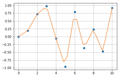
<練習問題 1>
以下のデータに対して、線形補間の計算をして、グラフを描いてください。
x = np.linspace(0, 10, num=11, endpoint=True)
x_ = np.linspace(0, 10, num=30, endpoint=True)
y = np.sin(x**2/5.0)
plt.plot(x,y,'o')
plt.grid(True)

f_1 = interpolate.interp1d(x, y,'linear')
plt.plot(x_, f_1(x_), '-')
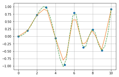
<練習問題 2>
2次元のスプライン補間をして上記のグラフに書き込んでください(2次元のスプライン補間はパラメタをquadraticとします。)
f_2 = interpolate.interp1d(x, y,'quadratic')
plt.plot(x, y, 'o', x_, f_1(x_), '-', x_, f_2(x_), '--')
plt.grid(True)
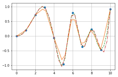
<練習問題 3>
3次元スプライン補間も加えてみましょう。
f_3 = interpolate.interp1d(x, y,'cubic')
plt.plot(x, y, 'o', x_, f_1(x_), '-', x_, f_2(x_), '--', x_, f_3(x_), '-.')
plt.grid(True)
5.3.2 線形代数:行列の分解
<練習問題 1>
以下の行列に対して、特異値分解をしてください。
B = np.array([[1,2,3],[4,5,6],[7,8,9],[10,11,12]])
print(B)
> [[ 1  2  3]
>  [ 4  5  6]
>  [ 7  8  9]
>  [10 11 12]]
# 特異値分解の関数linalg.svd
U, s, Vs = sp.linalg.svd(B)
m, n = B.shape

S = sp.linalg.diagsvd(s,m,n)

print("U.S.V* = \n",U@S@Vs)
> U.S.V* =
>  [[ 1.  2.  3.]
>  [ 4.  5.  6.]
>  [ 7.  8.  9.]
>  [10. 11. 12.]]
<練習問題 2>
以下の行列に対して、LU分解をして、 𝐴𝑥=𝑏 の方程式を解いてください。
# データの準備
A = np.identity(3)
print(A)
A[0,:] = 1
A[:,0] = 1
A[0,0] = 3
b = np.ones(3)
print(A)
print(b)
> [[1. 0. 0.]
>  [0. 1. 0.]
>  [0. 0. 1.]]
> [[3. 1. 1.]
>  [1. 1. 0.]
>  [1. 0. 1.]]
> [1. 1. 1.]
# 正方行列をLU分解する
(LU,piv) = sp.linalg.lu_factor(A)

L = np.identity(3) + np.tril(LU,-1)
U = np.triu(LU)
P = np.identity(3)[piv]

# 解を求める
x = sp.linalg.lu_solve((LU,piv),b)
print(x)
> [-1. 2. 2.]
5.3.3 積分と微分方程式
<練習問題 1>
以下の積分を求めてみましょう。\int_0^2 (x+1)^2 dx
integrate.quad(lambda x: (x+1)**2, 0, 2)
> (8.667, 0.000)
<練習問題 2>
cos関数の範囲 (0,𝜋) の積分を求めてみましょう。
from numpy import cos
integrate.quad(cos, 0, math.pi)
(0.000, 0.000)
5.3.4 最適化
<練習問題 1>
以下の関数が0となる解を求めましょう。\ f(x) = 5x -10
from scipy.optimize import fsolve

def f1(x):
    return 5 * x - 10

x = np.linspace(-100,100)
plt.plot(x,f1(x))
plt.plot(x,np.zeros(len(x)))
plt.grid(True)
plt.show()

x1 = fsolve(f1,0)
print(x1)

> [2.]
<練習問題 2>
以下の関数が0となる解を求めましょう。\ f(x) = x^3 - 2x^2 - 11x +12
from scipy.optimize import fsolve

def f2(x):
    return x**3 - 2 * x**2 - 11 * x + 12

x = np.linspace(-5,5)
plt.plot(x,f2(x))
plt.plot(x,np.zeros(len(x)))
plt.grid(True)
plt.show()

x1 = fsolve(f2,-99999)
x2 = fsolve(f2,0)
x3 = fsolve(f2,99999)
print(x1, x2, x3)

> [-3.] [1.] [4.]
5.4 総合問題
5.4.1 総合問題1
以下の行列に対して、コレスキー分解を活用して、𝐴𝑥=𝑏の方程式を解いてください。
A = np.array([[5, 1, 0, 1],
              [1, 9, -5, 7],
              [0, -5, 8, -3],
              [1, 7, -3, 10]])
b = np.array([2, 10, 5, 10])
L = sp.linalg.cholesky(A)

t = sp.linalg.solve(L.T.conj(), b)
x = sp.linalg.solve(L, t)

# 解答
print(x)
> [-0.051 2.157 2.01 0.098]
5.4.2 総合問題2
0≤𝑥≤1、0≤y≤1−x の三角領域で定義される以下の関数の積分値を求めてみましょう。\int_0^1 \int_0^{1-x} 1/(\sqrt{(x+y)}(1+x+y)^2) dy dx
from scipy import integrate

integrate.dblquad(lambda y, x:  1 / ((x + y)**(1/2) * (1 + x + y)**2), 0, 1, lambda x: 0, lambda x: 1-x)

# 関数をf(x, y)とした場合はどうすれば良いんだろう…
# def f(x,y):
#     1 / ((x + y)**(1/2) * (1 + x + y)**2)
# integrate.dblquad(f, 0, 1, lambda x: 0, lambda x: 1-x)
(0.285, 0.000)
5.4.3 総合問題3
以下の最適化問題をSicpyを使って解いてみましょう。\ min \ f(x) = x^2+1 \\ s.t. x \ge -1
from scipy.optimize import minimize

def f(x):
    return x**2 + 1

def constraint(x):
    return x+1

x0 = -1
con = {'type':'ineq','fun':constraint}
sol = minimize(f,x0,method='SLSQP',constraints=con)

print("x = " + str(sol.x) + " のとき、f(x)は最小値 " + str(sol.fun) + " を取る")

# memo
# conの"'type': 'eq'"は=0, "'type': 'ineq'"は=>0
> x = [2.22e-16] のとき、f(x)は最小値 1.0 を取る