scikit-FiniteDiff の適用例
1 次元 KdV (Korteweg–de Vries) 方程式の 2 Soliton 解
前回 は scikit-FiniteDiff を導入して、tutorial 例題を触ってみた。もう少し機能を見ていくために、大阪大学の講義資料 「数値解析法基礎」では Julia で扱われている KdV 方程式の問題に、Scikit-FiniteDiff を適用してみる。
http://www.cas.cmc.osaka-u.ac.jp/~paoon/Lectures/2019-8Semester-NA-basic/11-pde-method-of-line/#疑似-2-ソリトン解
%matplotlib inline
import numpy as np
import matplotlib.pyplot as plt
from skfdiff import Model, Simulation
Zarr module not found, ZarrContainer not available.
水深の浅い水面を進む波(浅水波)を記述する方程式として知られる Korteweg–de Vries (KdV) 方程式。
パラメータ 'a', 'b' は、scikit-FiniteDiff の例題のままで Model は作成し、パラメータの値の指定と初期値を変えてみる。
$
\frac{\partial U}{\partial t} + U,\frac{\partial U}{\partial x} = a,\frac{\partial^2 U}{\partial x^2} + b,\frac{\partial^3 U}{\partial x^3}
$
これを変形して、
$
\frac{\partial U}{\partial t} = -U,\frac{\partial U}{\partial x} + a,\frac{\partial^2 U}{\partial x^2} + b,\frac{\partial^3 U}{\partial x^3}
$
右辺を Model にする。
ここでは周期的境界条件を適用。
model = Model("-U * dxU + a * dxxU + b * dxxxU",
              "U(x)",
              ["a", "b"],
              boundary_conditions={("U", "x"):"periodic"}
             )
次に変数の範囲を定め、初期値を作る。刻み幅やパラメータは資料に準拠した。
$a = 0, b = - \epsilon^2$ として、$ \epsilon = 0.022$ を用いる。
x = np.linspace(0, 2, 200)
EPS = 0.022

def OneSoliton(height, center, x, epsilon=EPS):
    ''' 1 ソリトン解 '''
    d = np.sqrt(height / 12) / epsilon
    return height * np.cosh(d * (x - center)) ** (-2)
h1, c1 = 1., 0.5
h2, c2 = 0.5, 1.2

U = OneSoliton(h1, c1, x) + OneSoliton(h2, c2, x)
initial_fields = model.fields_template(x=x, U=U, a=0, b=-EPS ** 2)
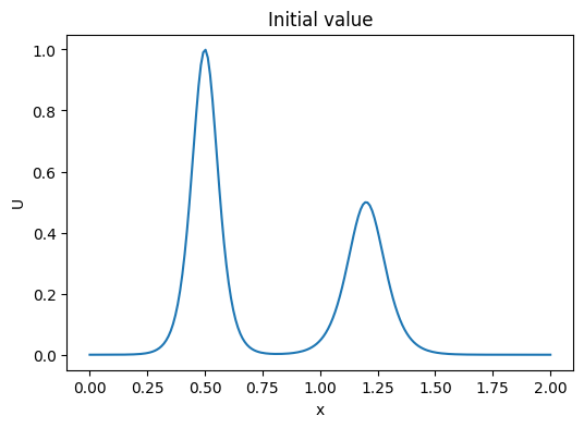
初期値の形を見てみよう
fig, ax = plt.subplots(1, 1, figsize=(6, 4))
ax.plot(x, U)
ax.set_xlabel("x")
ax.set_ylabel("U")
ax.set_title("Initial value")
Simulation を組み立て、 container を指定する
simulation = Simulation(model, initial_fields, dt=0.001, tmax=5., time_stepping=True)
container = simulation.attach_container()
解く
simulation.run()
a8a544 running: t: 5: : 5000it [02:14, 37.27it/s]


(5.0,
 <xarray.Dataset>
 Dimensions:  (x: 200)
 Coordinates:
   * x        (x) float64 0.0 0.01005 0.0201 0.03015 ... 1.97 1.98 1.99 2.0
 Data variables:
     U        (x) float64 0.08125 0.06985 0.06054 ... 0.1304 0.1113 0.09498
     a        int32 0
     b        float64 -0.000484)
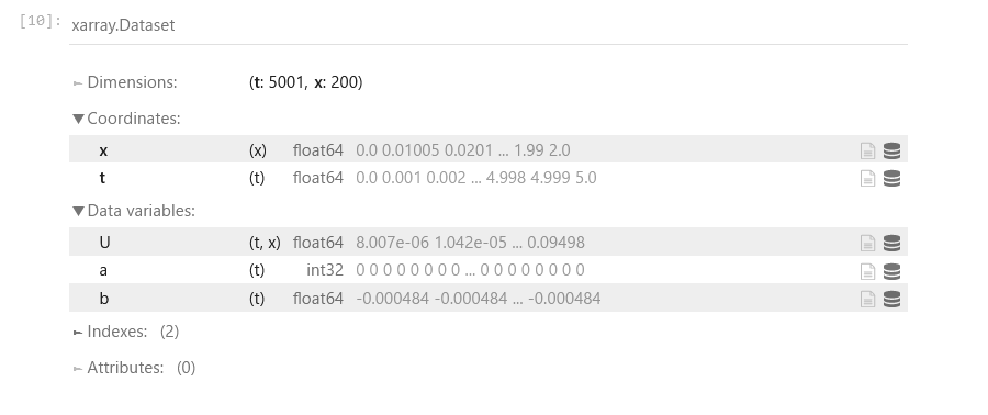
解、すなわち container の中身を確認
container.data
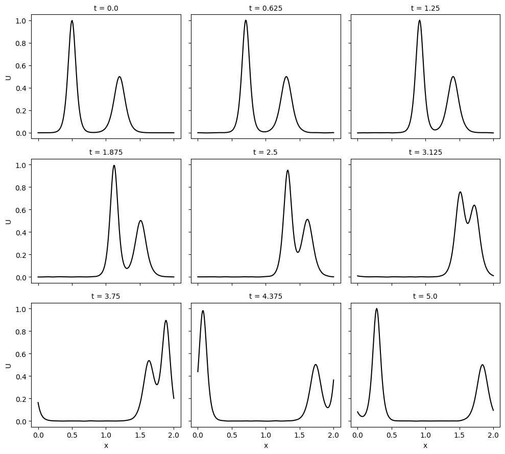
結果のプロットを見る
container.data.U[:: container.data.t.size // 8].plot(col="t", col_wrap=3, color="black")

二つのソリトンが波形を保って移動し、背が高く速いソリトンが小さいソリトンを追い越す挙動が見えている。
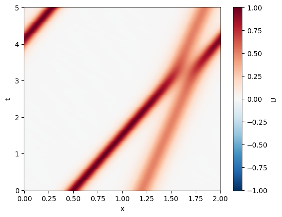
2D データをサンプリングして全体像が見えるようにプロットできる
container.data.U[::25].plot()
Backend に Numba を使ってみる
model_n = Model("-U * dxU + a * dxxU + b * dxxxU",
              "U(x)",
              ["a", "b"],
              boundary_conditions={("U", "x"):"periodic"},
              backend="numba")
simulation = Simulation(model_n, initial_fields, dt=0.001, tmax=5., time_stepping=True)
container = simulation.attach_container()
simulation.run()
  0%|                                                                                       | 0/4999.0 [00:00<?, ?it/s]C:\Users\natsu\py310\skfdiff\lib\site-packages\numba\core\ir_utils.py:2149: NumbaPendingDeprecationWarning: [1m
Encountered the use of a type that is scheduled for deprecation: type 'reflected list' found for argument 'subgrids' of function 'compute_jacobian_values'.

For more information visit https://numba.readthedocs.io/en/stable/reference/deprecation.html#deprecation-of-reflection-for-list-and-set-types

File "<string>", line 2:
<source missing, REPL/exec in use?>

  warnings.warn(NumbaPendingDeprecationWarning(msg, loc=loc))
C:\Users\natsu\py310\skfdiff\lib\site-packages\numba\core\ir_utils.py:2149: NumbaPendingDeprecationWarning: [1m
Encountered the use of a type that is scheduled for deprecation: type 'reflected list' found for argument 'subgrids' of function 'compute_jacobian_values'.

For more information visit https://numba.readthedocs.io/en/stable/reference/deprecation.html#deprecation-of-reflection-for-list-and-set-types

File "<string>", line 2:[0m
<source missing, REPL/exec in use?>

  warnings.warn(NumbaPendingDeprecationWarning(msg, loc=loc))
ef507c running: t: 5: : 5000it [01:44, 47.66it/s]


(5.0,
 <xarray.Dataset>
 Dimensions:  (x: 200)
 Coordinates:
   * x        (x) float64 0.0 0.01005 0.0201 0.03015 ... 1.97 1.98 1.99 2.0
 Data variables:
     U        (x) float64 0.08125 0.06985 0.06054 ... 0.1304 0.1113 0.09498
     a        int32 0
     b        float64 -0.000484)
Numba のコンパイル時の Warning が出るが、計算は進行している。手元の環境では、 numpy の 2 分 14 秒に対して 1 分 44 秒で計算を終えている。
container.data.U[:: container.data.t.size // 8].plot(col="t", col_wrap=3, color="black")
数値積分スキーム
'Rosenbrock-Wanner schemes'(個別の名前で指定), 'Theta', 'scipy_ivp' が選べる。
デフォルトでは、ルンゲクッタの一種の Rosenbrock-Wanner schemes の 6 次が適用されると記載。
Rosenbrock-Wanner schemes のバリエーションは、以下のもの
- "ROS2": Second order Rosenbrock scheme, without time stepping
- "ROS3PRw": Third order Rosenbrock scheme, with time stepping
- "ROS3PRL": 4th order Rosenbrock scheme, with time stepping
- "RODASPR": 6th order Rosenbrock scheme, with time stepping
ROS2 を指定した例
simulation = model_n.init_simulation(initial_fields, dt=.001, tmax=5,
    scheme="ROS2")  # Second order Rosenbrock scheme, without time stepping
Theta スキームを指定すると、以下のものが使える
- theta = 1: backward Euler
- theta = 0: forward Euler
- theta = 0.5: Crank-Nicolson
KdV では、forward Euler は発散しました。
Crank-Nikolson を指定:
simulation = model_n.init_simulation(initial_fields, dt=.001, tmax=5,
    scheme="Theta",  # using a theta scheme
    theta=0.5)  # Crank-Nicolson
scipy_ivp のバリエーション
詳しくは、https://docs.scipy.org/doc/scipy/reference/generated/scipy.integrate.solve_ivp.html を参照。
- "RK45" (default): Explicit Runge-Kutta method of order 5(4)
- "RK23": Explicit Runge-Kutta method of order 3(2)
- "DOP853": Explicit Runge-Kutta method of order 8
- Warning メッセージを見ると、指定が効いていないかもしれません
- "Radau": Implicit Runge-Kutta method of the Radau IIA family of order 5
- "BDF": Implicit multi-step variable-order (1 to 5) method based on a backward differentiation formula for the derivative approximation
- "LSODA": Adams/BDF method with automatic stiffness detection and switching
呼び出しの例
simulation = model_n.init_simulation(initial_fields, dt=.001, tmax=5,
    scheme="scipy_ivp",
    method="RK23")
まとめ
KdV 方程式のソリトン解を見るために、周期的境界条件を適用して、微分方程式のパラメータを書き換えて
数値解を求めた。 Numba バックエンドでの動作も試みた。
適用可能なスキームをひととおりリストアップして試した。
付録
全部一式の Jupyter notebook も作りました。各スキームの比較と、保存量のプロットも行っています。