Scikit-FiniteDiff を試用する

差分法の偏微分方程式ソルバー Scikit-FiniteDiff をインストールして使い始めています。¹

リンク先のイントロダクションに概要が書かれています。
sympy を使って離散化した方程式を作り、時間に対して Method of line の手法で解くとのこと。まずは、道具として使う観点で触っています。

環境構築

仮想環境を作って pip インストールして使い始めることができる。(Windows11, Python 3.10.11)

> cd %Userprofile% 
> .\AppData\Local\Programs\Python\Python310\python.exe -m venv --upgrade-deps skfdiff
> .\skfdiff\Scripts\Activate.ps1
> pip install scikit-fdiff[interactive,numba]
> ipython kernel install --user --name=py310_skfdiff

チュートリアル例題 'One dimension Korteweg–de Vries' を試す

%matplotlib inline

import numpy as np
# import pylab as pl
import matplotlib.pyplot as plt
from skfdiff import Model, Simulation

Zarr module not found, ZarrContainer not available. という Warning が出るけれど、先にすすむことはできる。

モデルを組み立てて解く

例題は、水深の浅い水面を進む波（浅水波）を記述する方程式として知られる Korteweg–de Vries (KdV) 方程式ということだが、
検索して上位で見つかる例では $a=0$ に相当する式が使われていることが多い。
ソリトン解で有名。

$
\frac{\partial U}{\partial t} + U\frac{\partial U}{\partial x} = a\frac{\partial^2 U}{\partial x^2} + b\frac{\partial^3 U}{\partial x^3}
$

これを変形して、
$
\frac{\partial U}{\partial t} = -U\frac{\partial U}{\partial x} + a\frac{\partial^2 U}{\partial x^2} + b\frac{\partial^3 U}{\partial x^3}
$

右辺を Model にする

model = Model("-U * dxU + a * dxxU + b * dxxxU", 
              "U(x)", 
              ["a", "b"]
             )

最初の引数が微分方程式で、第 2 の引数が未知数と独立変数を示す。第 3 の引数はパラメータである。関数の引数名としては、それぞれ 'evolution_equations', 'unknowns', 'parameters' となっている。

次に変数の範囲を定め、初期値を作る

x = np.linspace(-2, 6, 1000)

n = 20
U = np.log(1 + np.cosh(n) ** 2 / np.cosh(n * x) ** 2) / (2 * n)

initial_fields = model.fields_template(x=x, U=U, a=2e-4, b=1e-4)

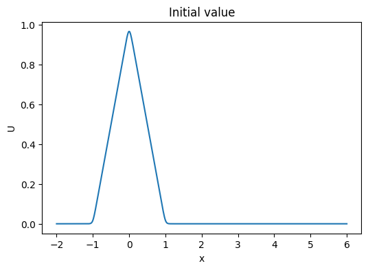
初期値の形を見てみよう

fig, ax = plt.subplots(1, 1, figsize=(6, 4))
ax.plot(x, U)
ax.set_xlabel("x")
ax.set_ylabel("U")
ax.set_title("Initial value")

これを使って、「シミュレーション」Simulation を組み立て、数値解析を実効することができる。
このとき経過を蓄積する container を指定できる。

simulation = Simulation(model, initial_fields, dt=0.05, tmax=10)
container = simulation.attach_container()

simulation.run()

(10.0,
 <xarray.Dataset>
 Dimensions:  (x: 1000)
 Coordinates:
   * x        (x) float64 -2.0 -1.992 -1.984 -1.976 ... 5.976 5.984 5.992 6.0
 Data variables:
     U        (x) float64 -5.501e-08 -5.347e-08 -4.966e-08 ... -0.04111 -0.04193
     a        float64 0.0002
     b        float64 0.0001)

結果の確認

simulation.run() は、最後のステップのデータだけを返すが、container は指定に応じて履歴データを保持できる。
container オブジェクトの使い方を見ていこう。
ちなみに simulation.attach_container() の返り値と simulation.container は同じものである。container.data に、x, t と解 U が保存されている。

container == simulation.container  ## True

container.data

結果のプロットを見る

container.data.U[:: container.data.t.size // 8].plot(col="t", col_wrap=3, color="black")

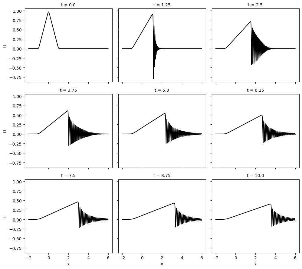
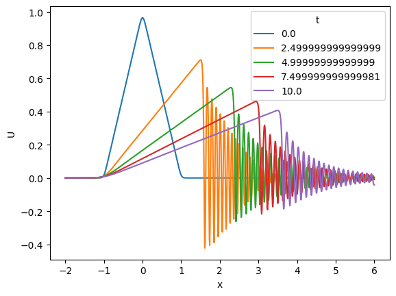
右側の短い波長で振動している部分がソリトン解ということのようだ。
ちなみに .plot の機能は、skfdiff 固有の機能ではなくて、 xarray の機能である。

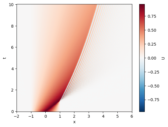
2D データを全部プロットさせることもできる

container.data.U.plot()

波形の重ね書きもできる

container.data.U.isel(t=slice(0, None, 50)).plot.line(hue="t")

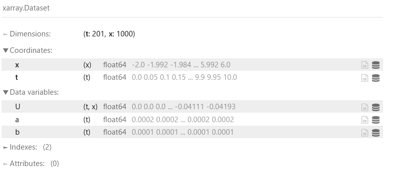
container.data.U.coords

xarray の container.data.U は、以下のような構造

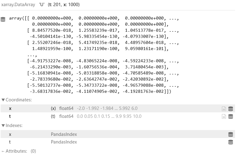
座標に直接アクセスすることができる。

container.data.U.coords

Coordinates:
  * x        (x) float64 -2.0 -1.992 -1.984 -1.976 ... 5.976 5.984 5.992 6.0
  * t        (t) float64 0.0 0.05 0.1 0.15 0.2 0.25 ... 9.8 9.85 9.9 9.95 10.0

まとめと今後

解のハンドリングを自分で考えるより、フレームワークを活用すると低コストでソルバーを使えそう。
パラメータを変えて、ソリトン解の文献との比較。
別の微分方程式を入れて、境界条件の指定や、hook, 風上差分指定などの機能を見ていきたい。
覚書: 差分法の他のツールとして、見つけたもの
- py-pde
- Devito
- 一般的に言えば、任意の領域で解ける FEM の方が汎用性は高い。skfdiff のイントロダクションページで論じられている

付録

全部一式の Jupyter notebook も作りました

https://joss.theoj.org/papers/10.21105/joss.01356 ↩

scikit-FiniteDiff を使ってみる