This article shows the fundamentals of using CUDA for accelerating convolution operations. Since convolution is the important ingredient of many applications such as convolutional neural networks and image processing, I hope this article on CUDA would help you to know about convolution and its parallel implementation. I believe in that writing software is a powerful way to understand and demonstrate what one would like to realize.
If you are familiar with a convolution operation and CUDA, you can directory access the example code at github, in which accelerated image filtering is implemented by C++ and CUDA: https://github.com/NaoyukiIchimura/cuda_image_filtering_global. In this version, only global memory of a GPU is used.
1. A convolution operation for an image
Let's assume that $f\left(x,y\right)$ is an image where $\left(x, y\right)$ represent a pixel coordinate in the coordinate system shown on the left in Fig.1, and the width and height of the image are denoted by $W$ and $H$. A convolution operation for the image can be represented by the following equation:
h\left(x,y\right)=\sum_{\alpha=-S}^S \sum_{\beta=-S}^S f\left(x+\alpha,y+\beta\right)g\left(\alpha,\beta\right), \tag{1}
where, $g\left(\alpha,\beta\right)$ is a filter with the coordinate system shown on the right in Fig.1, and $S$ determines the size of the filter as $\left(2S+1\right)\times\left(2S+1\right)$. Figure 2 shows an example of the convolution operation of a 3 $\times$ 3 filter at the coordinate $\left(x,y\right)=\left(2,2\right)$. In the 3 $\times$ 3 neighborhood of the coordinate, the pixel values are multiplied by the corresponding filter coefficients and the results of the multiply operations are added. That is, a multiply-add operation is performed in the neighborhood.
 *Figure 1. A coordinate system of an image and a filter.*
 *Figure 2. An example of a convolution operation.*
Note that there is no causality caused by time among pixel data in an image, the order of the multiply operations can be arbitrary as long as the correspondences between pixel data and filter coefficients are correctly kept. For example, the convolution operation can be represented by the following equation as well:
h\left(x,y\right)=\sum_{\alpha=-S}^S \sum_{\beta=-S}^S f\left(x-\alpha,y-\beta\right)g\left(-\alpha,-\beta\right).\tag{2}
The filtering result is obtained by performing the convolution operation for every pixel in the image, i.e., for all the coordinates $\left(x,y\right),$ $x=0,\dots,W-1,$ $y=0,\dots,H-1$. Since corresponding pixels cannot be found out for some filter coefficients at the edges of the image as shown in Fig.3, extra pixels are added to the sides of the image. Appending pixels is called padding and Figure 4 shows typical examples of it, zero padding and replication padding. The size of padding is normally $S$ for the filter with the size $\left(2S+1\right)\times\left(2S+1\right)$.
 *Figure 3. The convolution operations at the edges of the image.*
 *Figure 4. Examples of padding; zero padding and replication padding.*
2. Graphics processing units (GPUs) and compute unified data architecture (CUDA)
The convolution operation of Eq.(1) can be independently performed for all the coordinates $\left(x,y\right),$ $x=0,\dots,W-1,$ $y=0,\dots,H-1$, because the result of a coordinate do not affect the results of the others. Thus parallel computation is very useful to shorten the computation time of filtering. Using graphics processing units (GPUs) and the computing architecture called compute unified data architecture (CUDA) developed by the NVIDIA corporation is an effective way to realize parallel computation. The brief introduction of GPUs and CUDA is shown below. If you would like to install CUDA Toolkit to a computer with a CUDA enable GPU, the page I wrote might help you: Installing CUDA 9.2, TensorFlow, Keras and PyTorch on Fedora 27 for Deep Learning.
2-1. The overview of the architecture of a GPU.
Figure 5 shows the overview of the architecture of a GPU. There are multiprocessors (MPs) in a GPU and each MP has CUDA cores. You can check how many MPs and CUDA cores your GPU has by running the command deviceQuery distributed with the CUDA sample programs in the CUDA Toolkit. Figure 6 shows the output of the command for the GPU, GeForce GTX 1080 Ti. The fifth line of the output shows that there are 28 MPs and 128 CUDA cores/MP in the GPU and thus 28$\times$128=3584 CUDA cores can be utilized. Parallel computing is performed by assigning a large number of threads to CUDA cores.
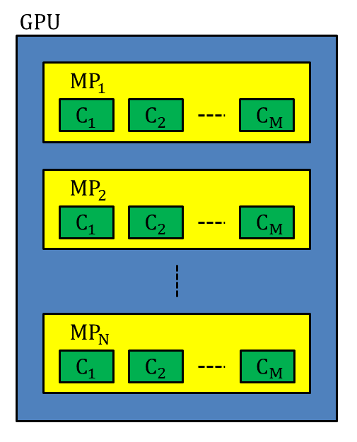 *Figure 5. The overview of the architecture of a GPU. MP and C stand for a multiprocessor and a CUDA core, respectively.*
Device 0: "GeForce GTX 1080 Ti"
  CUDA Driver Version / Runtime Version          9.2 / 9.2
  CUDA Capability Major/Minor version number:    6.1
  Total amount of global memory:                 11178 MBytes (11721506816 bytes)
  (28) Multiprocessors, (128) CUDA Cores/MP:     3584 CUDA Cores
  GPU Max Clock rate:                            1582 MHz (1.58 GHz)
  Memory Clock rate:                             5505 Mhz
  Memory Bus Width:                              352-bit
  L2 Cache Size:                                 2883584 bytes
  Maximum Texture Dimension Size (x,y,z)         1D=(131072), 2D=(131072, 65536), 3D=(16384, 16384, 16384)
  Maximum Layered 1D Texture Size, (num) layers  1D=(32768), 2048 layers
  Maximum Layered 2D Texture Size, (num) layers  2D=(32768, 32768), 2048 layers
  Total amount of constant memory:               65536 bytes
  Total amount of shared memory per block:       49152 bytes
  Total number of registers available per block: 65536
  Warp size:                                     32
  Maximum number of threads per multiprocessor:  2048
  Maximum number of threads per block:           1024
  Max dimension size of a thread block (x,y,z): (1024, 1024, 64)
  Max dimension size of a grid size    (x,y,z): (2147483647, 65535, 65535)
  Maximum memory pitch:                          2147483647 bytes
  Texture alignment:                             512 bytes
  Concurrent copy and kernel execution:          Yes with 2 copy engine(s)
  Run time limit on kernels:                     No
  Integrated GPU sharing Host Memory:            No
  Support host page-locked memory mapping:       Yes
  Alignment requirement for Surfaces:            Yes
  Device has ECC support:                        Disabled
  Device supports Unified Addressing (UVA):      Yes
  Device supports Compute Preemption:            Yes
  Supports Cooperative Kernel Launch:            Yes
  Supports MultiDevice Co-op Kernel Launch:      Yes
  Device PCI Domain ID / Bus ID / location ID:   0 / 21 / 0
  Compute Mode:
     < Default (multiple host threads can use ::cudaSetDevice() with device simultaneously) >
Figure 6. The output of the command "deviceQuery" for the GPU, GeForce GTX 1080 Ti. The information obtained by the command is important to write a program using CUDA.
2-2. Dividing data for parallel computing using CUDA
In software implementations, the convolution operations for filtering can be realized by a nested loop structure. An example program written by C++ is as follows:
template <typename T>
int imageFiltering( const T *h_f, const unsigned int &paddedW, const unsigned int &paddedH,
                    const T *h_g, const int &S,
                    T *h_h, const unsigned int &W, const unsigned int &H )
{

    // Set the padding size and filter size
    unsigned int paddingSize = S;
    unsigned int filterSize = 2 * S + 1;

    // The loops for the pixel coordinates
    for( unsigned int i = paddingSize; i < paddedH - paddingSize; i++ ) {
        for( unsigned int j = paddingSize; j < paddedW - paddingSize; j++ ) {

            // The multiply-add operation for the pixel coordinate ( j, i )
            unsigned int oPixelPos = ( i - paddingSize ) * W + ( j - paddingSize );
            h_h[oPixelPos] = 0.0;
            for( int k = -S; k <=S; k++ ) {
                for( int l = -S; l <= S; l++ ) {
                    unsigned int iPixelPos = ( i + k ) * paddedW + ( j + l );
                    unsigned int coefPos = ( k + S ) * filterSize + ( l + S );
                    h_h[oPixelPos] += h_f[iPixelPos] * h_g[coefPos];
                }
            }

        }
    }

    return 0;

}
In the code, the argument h_f is an input image after padding is applied, paddedW and paddedH are the size of the padded image, h_g is a filter, S determines the sizes of the filer and padding, h_h is a filtered image, and W and H are the size of an input image. Note that padding of $S$ pixels for an input image is assumed. Allocated one-dimensional (1D) arrays are used for the images and the filter, because using 1D arrays is convenient to allocate a memory space on a GPU. Note that accessing the 2D data in a 1D array is a little bit tricky; the access pattern of a 2D array denoted by a[i][j] corresponds to one of a 1D array denoted by a[ i * X + j ] where X is the width of the 2D data.
The loops with the counters i and j are for the pixel coordinates of the padded image, and ones with the counters k and l are for the convolution operations performed in the $\left(2S+1\right)\times\left(2S+1\right)$ neighborhood of all the pixel coordinates. As we can see from this code, the convolution operations can be parallelized because the operation for a pixel coordinate is independent from the others.
In order to parallelize the convolution operations using CUDA, an image is divided into blocks by a grid as shown in Fig. 7. In implementations using CUDA, MPs in a GPU are assigned to the blocks and threads executed by CUDA cores are assigned to the pixels in each block automatically. Therefore, what we have to do is writing the program for the threads to perform the convolution operations. CUDA C/C++ that is an extension of C/C++ for parallel computing is used to write the program.
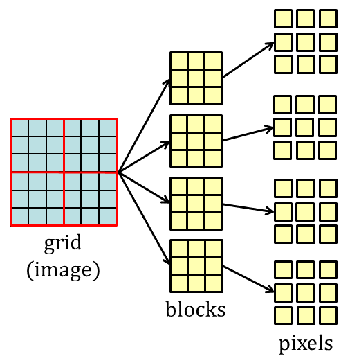 *Figure 7. The hierarchy of data defined by a grid.*
3. Writing CUDA C/C++ program for convolution operations
The CUDA C/C++ program for parallelizing the convolution operations explained in this section constitutes the following procedures:
(1) Transferring an image and a filter from a host to a device.
(2) Setting the execution configuration.
(3) Calling the kernel function for the convolution operations.
(4) Transferring the filtering result from the device to the host.
3-1. Transferring an image and a filter from a host to a device
A GPU is connected to a computer via a bus such as the PCI express bus. A computer and a GPU are called a host and a device respectively, and have their own memory. An image and a filter are loaded to host memory by host code and they have to be transferred to device memory to carry out parallel processing. In this article, a type of device memory called global memory is used. Global memory is also referred to as graphics memory and the total amount of it can be checked by the command deviceQuery as shown in Fig.6.
In the example program shown in section 2-2 and the following program, the prefix h_ of the variables represents that the variables are in host memory. On the other hand, the prefix d_ of the variables in the following programs shows that the variables are in global memory.
Transferring variables between a host and a device is executed by the function cudaMemcpy() of CUDA API as shown in the following sample program:
// Allocate the memory space for an image with the size 1920x1080 on a host
float *h_tmpF;
unsigned int W = 1920;
unsigned int H = 1080;
h_tmpF = new float[ W * H ];

// Read the image from the file, scene2_fullHD.png
readImage( h_tmpF, "scene2_fullHD.png" );

// Allocate the memory space for a 3x3 filter on a host
float *h_g;
int S = 1; // the parameter determines the size of a filter; note the signed type
unsigned int filterSize = 2 * S + 1;
h_g = new float[ filterSize * filterSize ];

// Read the coefficients of a filter from the file, gradient_filter.dat
readFilter( h_g, "gradient_filter.dat" );

// Perform padding for the image
// Note that the padding size is S.
unsigned int paddedW = W + 2 * S;
unsigned int paddedH = H + 2 * S;
float *h_f;
h_f = new float[ paddedW * paddedH ];
replicationPadding( h_tmpF, W, H,
                    S,
                    h_f, paddedW, paddedH );

// Allocate the memory space for the padded image on a device
float *d_f;
unsigned int paddedImageSizeByte = paddedW * paddedH * sizeof(float);
cudaMalloc( reinterpret_cast<void **>(&d_f), paddedImageSizeByte );

// Transfer the padded image from a host to a device
cudaMemcpy( d_f, h_f, paddedImageSizeByte, cudaMemcpyHostToDevice ); // Host to Device

// Allocate the memory space for the filter on a device
float *d_g;
unsigned int filterKernelSizeByte = filterSize * filterSize * sizeof(float);
cudaMalloc( reinterpret_cast<void **>(&d_g), filterKernelSizeByte );

// Transfer the filter from a host to a device
cudaMemcpy( d_g, h_g, filterKernelSizeByte, cudaMemcpyHostToDevice ); // Host to Device
The function cudaMalloc() is used to allocate a memory space on a device, while new is used for a host.
Note that since transferring data between a host and a device may not be so fast compared to computation itself due to the bandwidth limitation of a bus between a CPU and a GPU, you have to consider the effectiveness of introducing GPU including the elapsed time for data transfer.
3-2. Setting the execution configuration
The parameters defining the size of a grid and the number of threads assigned to a block are called the execution configuration. The execution configuration is set using the dim3 variable in CUDA C/C++. The variable is a vector containing unsigned int variables and its maximum dimension is 3.
If the width and height of a block are blockW and blockH, the grid on the image has the size $\lceil$ H/blockH $\rceil$$\times$$\lceil$ W/blockW $\rceil$. The declaration of the variable for defining the 2D grid size is:
const dim3 grid( iDivUp( W, blockW ), iDivUp( H, blockH ) );
where, iDivUp() is an inline function of the ceiling function for unsigned int variables:
inline unsigned int iDivUp( const unsigned int &a, const unsigned int &b ) { return ( a%b != 0 ) ? (a/b+1):(a/b); }.
The number of threads for a block is assigned by the same manner of the grid. That is, the width and height of a thread block are set using a dim3 variable.
const dim3 threadBlock( blockW, blockH );
In the above case, the number of threads is equal to the number of pixels in a block. Thus the convolution operations for a block are fully parallelized by threads. Note that since the number of threads per block is limited, e.g., the maximum number is 1024 in GeForce GTX 1080 Ti as shown in Fig.6, sequential processing should be incorporated if the number of pixels in a block exceeds the maximum number of threads. In the evaluation shown in section 4, the block size was set:
const unsigned int blockW = 32;
const unsigned int blockH = 32;
which means that the maximum number of threads (32$\times$32=1024) were launched for a block.
The 2D assignment of the size of the grid and one of the thread block enable us to discriminate the thread for each pixel coordinate in the kernel function explained in the next section.
3-3. Calling the kernel function for the convolution operations
A function callable from host code and executed on a device is called a kernel. In this article, a kernel is referred to as a kernel function to avoid the confusion of it with the other kernels used in pattern recognition and image processing.
The kernel function imageFilteringKernel() for image filtering is invocated in host code as follows:
float *d_h; // the filtering result
unsigned int imageSizeByte = W * H * sizeof(float);
cudaMalloc( reinterpret_cast<void **>(&d_h), imageSizeByte );

imageFilteringKernel<<<grid,threadBlock>>>( d_f, paddedW, paddedH,
                                            d_g, S,
                                            d_h, W, H );

cudaDeviceSynchronize();
The execution configuration is given to the kernel function by the <<<...>>> syntax. The function cudaDeviceSynchronize() is for waiting to complete all the processing performed on a GPU. If the function is removed, the host code is executed without waiting, which enable us parallel processing using both a CPU and a GPU. However, you cannot use the filtering result in host code safely.
The kernel function that requires the __global__ declaration specifier can be written as follows:
template <typename T>
__global__ void imageFilteringKernel( const T *d_f, const unsigned int paddedW, const unsigned int paddedH,
                                      const T *d_g, const int S,
                                      T *d_h, const unsigned int W, const unsigned int H )
{

    // Set the padding size and filter size
    unsigned int paddingSize = S;
    unsigned int filterSize = 2 * S + 1;

    // Set the pixel coordinate
    const unsigned int j = blockIdx.x * blockDim.x + threadIdx.x + paddingSize;
    const unsigned int i = blockIdx.y * blockDim.y + threadIdx.y + paddingSize;

    // The multiply-add operation for the pixel coordinate ( j, i )
    if( j >= paddingSize && j < paddedW - paddingSize && i >= paddingSize && i < paddedH - paddingSize ) {
        unsigned int oPixelPos = ( i - paddingSize ) * W + ( j - paddingSize );
        d_h[oPixelPos] = 0.0;
        for( int k = -S; k <=S; k++ ) {
            for( int l = -S; l <= S; l++ ) {
                unsigned int iPixelPos = ( i + k ) * paddedW + ( j + l );
                unsigned int coefPos = ( k + S ) * filterSize + ( l + S );
                d_h[oPixelPos] += d_f[iPixelPos] * d_g[coefPos];
            }
        }
    }

}
Note that the type of a kernel function must be void and passing arguments by references cannot be used. The major difference between the function imageFiltering() in Section 2-2 for a CPU and the kernel function is that the kernel function has no nested loop structure for the pixel coordinates assigned as (j, i). The pixel coordinates are computed using the built-in variables, namely blockIdx, blockDim and threadIdx instead. The variable blockIdx is used to identify the coordinate of each block in the grid, the variable blockDim gives us the dimension of the block, and the variable threadIdx is used to identify a unique thread ID assigned to a pixel in the block. These variables can have three components:
blockIdx.x, blockIdx.y, blockIdx.z
blockDim.x, blockDim.y, blockDim.z
threadIdx.x, threadIdx.y, threadIdx.z
In this case, the 2D grid and 2D thread block are defined by the execution configuration, we can compute the coordinates of the blocks and thread IDs using blockIdx.x, blockIdx.y, blockDim.x, blockDim.y, threadIdx.x and threadIdx.y.
As the grid is defined by the dim3 variable grid( iDivUp( W, blockW ), iDivUp( H, blockH ) ), the components blockIdx.x and blockIdx.y vary within [ 0, iDivUp( W, blockW ) - 1 ] and [ 0, iDivUp( H, blockH ) - 1 ], respectively. Similary, the components threadIdx.x and threadIdx.y vary within [ 0, blockW-1 ] and [ 0, blockH-1 ] because of the definition threadBlock( blockW, blockH ). The values of these components are automatically given by a GPU and thus iDivUp( W, blockW )$\times$iDivUp( H, blockH )$\times$blockW$\times$blockH kernel functions are invoked simultaneously for parallel processing. In the sample program, the size of the input image is 1920$\times$1080. If we set blockW=32 and blockH=32, the grid size is 60$\times$34 and the size of the thread block is 32$\times$32. Therefore, 60$\times$34$\times$32$\times$32=2,088,960 kernel functions are executed.
The coordinates of the blocks in the image coordinate system shown by the yellow pixels in Fig.8 are computed by blockIdx and blockDim as:
( blockIdx.x * blockDim.x, blockIdx.y * blockDim.y ),
where, blockDim.x=blockW and blockDim.y=blockH. The pixel coordinates in a block are given by threadIdx:
( threadIdx.x, threadIdx.y ).
Thus the pixel coordinates with respect to the image coordinate system represented by (j, i) are given by:
j = blockIdx.x * blockDim.x + threadIdx.x + paddingSize,
i = blockIdx.y * blockDim.y + threadIdx.y + paddingSize.
Note that padding size have to be compensated. Invoked kernel functions correspond to the pixel coordinates computed by the above equations. The relationship between the pixel coordinates and the built-in varibles is summarized in Fig.9.
 *Figure 8. The coordinates of the blocks in the image coordinate system shown by the yellow pixels are computed by the build-in variables, blockIdx and blockDim. The pixel coordinates in a block are given by the build-in variable, threadIdx.*
 *Figure 9. A summary of the relationship between the pixel coordinates and build-in variables.*
Since blocks do not always cover an image regularly as shown in Fig.10, some of threads corresponding to the coordinates outside of an image are not used. In the kernel function, excluding such threads is carried out by the following statement:
if( j >= paddingSize && j < paddedW - paddingSize && i >= paddingSize && i < paddedH - paddingSize )
 *Figure 10. Irregular blocks for parallel processing. Some of threads corresponding to the coordinates outside of an image are not used.*
As we can see from the kernel function, the essential code for the convolution operation is the same for a host; the nested loop structure for the image coordinates is merely removed. That is, removing loops is the basic strategy to write a kernel function by porting a program for a host.
3-4. Transferring the filtering result from the device to the host
In order to save the filtering result as an image, the variable d_h in the kernel function have to be transferred from the device to the host. Transferring the filtering result can be done by the function cudaMemcpy() as follows:
float *h_h;
h_h = new float[ W * H ];

cudaMemcpy( h_h, d_h, imageSizeByte, cudaMemcpyDeviceToHost ); // Device to Host
4. Evaluating the performance of the kernel function
The evaluation on how the kernel function contributes to accelerate the convolution operations was performed using a horizontal gradient filter. The following 3x3 and 5x5 filters were used:
[3x3]
-0.112737 0.0 0.112737
-0.274526 0.0 0.274526
-0.112737 0.0 0.112737

[5x5]
-0.003776 -0.010199 0.0 0.010199 0.003776
-0.026786 -0.070844 0.0 0.070844 0.026786
-0.046548 -0.122572 0.0 0.122572 0.046548
-0.026786 -0.070844 0.0 0.070844 0.026786
-0.003776 -0.010199 0.0 0.010199 0.003776
The filter coefficients were obtained from the paper:
S. Ando: Consistent gradient operators, IEEE Trans. PAMI, Vol.22, No.3, pp.252-265, 2000.
 *Figure 11. The image used in the evaluation of the kernel function.*
The image used in the evaluation is shown in Fig.11. The size of the image is 1920x1080. The filters were applied to the Y component of the image which was computed by the equation:
Y = 0.2126R + 0.7152G + 0.0722B,
where, $R$, $G$ and $B$ represent RGB color components. That is, the image was converted to a grayscale image.
The effectiveness of introducing GPU was evaluated by computation times of the CPU and GPU, Intel Xeon Gold 5122 and NVIDIA GeForce GTX 1080 Ti. The function gettimeofday() was used to measure computation times. Table 1 shows the computation times of the CPU and the GPU for filtering and data transfer. As we can see from the table, the convolution operations for filtering was clearly accelerated by the parallel processing; the GPU was 36.6X and 31.4X faster than the CPU for the 3x3 and 5x5 filters, respectively. However, transferring the image and filter coefficients had to be performed for the GPU, the overall rates of speed-up were reduced to 3.8x and 7.5x. Note the loss of efficiency due to data transfer when you apply the GPU computing.
| Filter size | CPU (Filtering) |
GPU (Filtering) |
GPU (Transfer) |
Speed-up (Filtering) |
Speed-up (Overall) |
|---|---|---|---|---|---|
| 3x3 | 19.78 | 0.54 | 4.62 | 36.6X | 3.8X |
| 5x5 | 45.90 | 1.46 | 4.70 | 31.4X | 7.5X |
| Table 1. The computation times of the CPU and the GPU for filtering and data transfer. The unit is [ms]. Although the computation times varied by trial due to the non-real time property of OS (Linux), the GPU was always faster than the CPU as shown in this table. |
Allocating and using write-combined memory (WC memory) which is a type of page-locked host memory is a way to make data transfer efficient. The function cudaHostAlloc() is used to allocate WC memory instead of new as the following code. However, reading WC memory by a CPU is often inefficient and using it on a host makes processing very slow as a result. Thus using WC memory is advisable if you use it as a buffer for transfer.
// Perform padding for the image
// Note that the padding size is S.
unsigned int paddedW = W + 2 * S;
unsigned int paddedH = H + 2 * S;
float *h_f;
unsigned int paddedImageSizeByte = paddedW * paddedH * sizeof(float);
cudaHostAlloc( reinterpret_cast<void **>(&h_f), paddedImageSizeByte, cudaHostAllocWriteCombined );
replicationPadding( h_tmpF, W, H,
                    S,
                    h_f, paddedW, paddedH );

// Allocate the memory space for the padded image on a device
float *d_f;
cudaMalloc( reinterpret_cast<void **>(&d_f), paddedImageSizeByte );

// Transfer the padded image from a host to a device
cudaMemcpy( d_f, h_f, paddedImageSizeByte, cudaMemcpyHostToDevice ); // Host to Device

...

// Free the host memory space
cudaHostFree( h_f );
 *The result of the 3x3 filter.*
 *The result of the 5x5 filter.*
Figure 12. The results of filtering performed by the GPU. The postprocessing was applied to the outputs of the filters to make the images.
Figure 12 represents the filtering results by the GPU. To make the images in this figure, the following postprocessing was applied to the outputs of the filters: taking absolute values of the outputs and normalizing the absolute values to [0,255]. The results were identical to the results obtained by the CPU. However, the --fmad option of the CUDA compiler driver nvcc had to be set as --fmad=false, which disables the contraction of floating-point multiplies and adds into floating-point multiply-add operations (FMAD). For the case where the option was true, the mean-squared error between the filtering results of the CPU and GPU was $1.86\times 10^{-3}$. Note that the default value of --fmad is true and using the option --use_fast_math implies --fmad=true.
You can find the code used to compute the results at https://github.com/NaoyukiIchimura/cuda_image_filtering_global.
The evaluation of this section demonstrates that although data transfer is required, using CUDA is useful to accelerate the convolution operations. The efficiency of GPU computing can be improved by utilizing the memory hierarchy of a GPU, for which the part 2 of this article is written: https://qiita.com/naoyuki_ichimura/items/519a4b75f57e08619374.