はじめに

前回はGraphNetを使って「とにかく５を出力する」ように学習しました。今回は、ノードやエッジの値を足し算する学習をしてみようと思います。

環境などは前回と同じです。

足し算を学習する

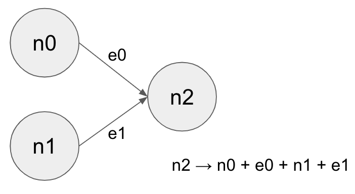
今回は、下の図のようなグラフを作って、全部のノードやエッジの値を足し合わせるように学習できるかやってみます。

コード

import numpy as np
import sonnet as snt
import graph_nets as gn
import tensorflow as tf
import matplotlib.pyplot as plt
from pprint import pprint

%matplotlib inline

tf.reset_default_graph()


def create_data_dict(n0=0., n1=0., e0=0., e1=0.):
    data_dict = dict(
        nodes=[[n0], [n1], [0.]], # node attrs (n0, n1, n2)
        edges=[[e0], [e1]],    # edge attrs (e0, e1)
        globals=[0.],
        receivers=[2, 2],
        senders=[0, 1],
        n_node=3,
        n_edge=2,
    )
    return data_dict

def create_graphs_tuple(n0=0., n1=0., e0=0., e1=0.):
    return gn.utils_tf.data_dicts_to_graphs_tuple([create_data_dict(n0, n1, e0, e1)])

def create_graphs_tuple_with_placeholder():
    # data_dicts の 値の部分を全てplaceholderに置き換えてくれる便利関数。他にも似たような便利関数がある。
    return gn.utils_tf.placeholders_from_data_dicts([create_data_dict()])

graph_in = create_graphs_tuple_with_placeholder()
graph_in = gn.utils_tf.make_runnable_in_session(graph_in)  # egdes: None -> edges: tf.no_op() みたいな変換をしている

# GraphNet を作る
graph_net_module = gn.modules.GraphNetwork(
    edge_model_fn=lambda: snt.nets.MLP([1]),
    node_model_fn=lambda: snt.nets.MLP([1]),
    global_model_fn=lambda: lambda x: x,
)

# GraphNet に入力グラフ(GraphsTuple)を入れて、出力グラフ(GraphsTuple)を作る
output_graphs = graph_net_module(graph_in)

# 正解はfeed_dictで渡すことにするので placeholderにしておく
target_value_ph = tf.placeholder(tf.float32)
# 最後のノードを決め打ちで対象とする。
loss_op_tr = (output_graphs.nodes[-1] - target_value_ph)**2  

# Optimizer.
learning_rate = 1e-4
optimizer = tf.train.MomentumOptimizer(learning_rate, momentum=0.9)
step_op = optimizer.minimize(loss_op_tr)

# Init Session
try:
  sess.close()
except NameError:
  pass
sess = tf.Session()
sess.run(tf.global_variables_initializer())


# Training
# feed_dict で placeholder にグラフを動的に注入しているのがややポイント
loss_history = []
for _ in range(1000):
    n0, n1, e0, e1 = np.random.random(4) * 10 - 5
    train_values = sess.run({
      "loss": loss_op_tr,
      "step": step_op,
      "outputs": output_graphs,
    }, feed_dict={
      graph_in.nodes: [[n0], [n1], [0.]],
      graph_in.edges: [[e0], [e1]],
      graph_in.globals: [[0]],
      graph_in.receivers: [2, 2],
      graph_in.senders: [0, 1],
      graph_in.n_node: [3],
      graph_in.n_edge: [2],
      target_value_ph: [n0+e0 + n1+e1],
    })
    loss_history.append(train_values['loss'])

plt.plot(loss_history)

ポイント

入力のGraphをplaceholderで置き換えると、feed_dictで動的に内容を変えられる

以下のようにすると、値が全て tf.placeholder な GraphsTupleができます。

def create_graphs_tuple_with_placeholder():
    # data_dicts の 値の部分を全てplaceholderに置き換えてくれる便利関数。他にも似たような便利関数がある。
    return gn.utils_tf.placeholders_from_data_dicts([create_data_dict()])

create_graphs_tuple_with_placeholder() のreturnは、以下のようになります。

GraphsTuple(
  nodes=<tf.Tensor 'placeholders_from_data_dicts_5/nodes:0' shape=(?, 1) dtype=float32>, 
  edges=<tf.Tensor 'placeholders_from_data_dicts_5/edges:0' shape=(?, 1) dtype=float32>, 
  receivers=<tf.Tensor 'placeholders_from_data_dicts_5/receivers:0' shape=(?,) dtype=int32>, 
  senders=<tf.Tensor 'placeholders_from_data_dicts_5/senders:0' shape=(?,) dtype=int32>, 
  globals=<tf.Tensor 'placeholders_from_data_dicts_5/globals:0' shape=(?, 1) dtype=float32>, 
  n_node=<tf.Tensor 'placeholders_from_data_dicts_5/n_node:0' shape=(1,) dtype=int32>, 
  n_edge=<tf.Tensor 'placeholders_from_data_dicts_5/n_edge:0' shape=(1,) dtype=int32>
)

そして、Trainingのときに、値や正解を差し込むと色々なケースで学習ができます。

    train_values = sess.run({
      "loss": loss_op_tr,
      "step": step_op,
      "outputs": output_graphs,
    }, feed_dict={
      graph_in.nodes: [[n0], [n1], [0.]],
      graph_in.edges: [[e0], [e1]],
      graph_in.globals: [[0]],
      graph_in.receivers: [2, 2],
      graph_in.senders: [0, 1],
      graph_in.n_node: [3],
      graph_in.n_edge: [2],
      target_value_ph: [n0+e0 + n1+e1],
    })

結果

Loss

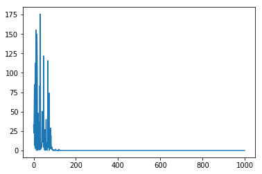
ちゃんと減ってます。

計算させてみる

こんな感じで計算させてみると、

n0, n1, e0, e1 = 0.1, 1.29, -0.3, 0.87
test_graph = create_graphs_tuple(n0, n1, e0, e1)
correct_value = n0+e0 + n1+e1
test_out = sess.run(graph_net_module(test_graph))
print(f"graph_output={test_out.nodes[2]} : correct_value={correct_value}")

まあ、概ね正解と言える結果が返ってきました。

graph_output=[1.9599973] : correct_value=1.96

しかし、結構差が出ることがあって、MLPのレイヤーや運によってはなんかひどくズレることもよくあります。

違う構造のGraphで計算させてみる

２ノード → 1ノードで学習させたGraphNetで、３ノード → 1ノードを計算させるとどうなるのでしょうか。

やってみます。

data_dict = dict(
    nodes=[[3.4], [-0.5], [-0.5], [0.]],
    edges=[[-0.1], [0.3], [1.4]], 
    globals=[0.],
    receivers=[3, 3, 3],
    senders=[0, 1, 2],
    n_node=4,
    n_edge=3,
)

g = gn.utils_tf.data_dicts_to_graphs_tuple([data_dict])
correct_value = 3.4 - 0.1 - 0.5 + 0.3 - 0.5 + 1.4
test_out = sess.run(graph_net_module(g))
print(f"graph_output={test_out.nodes[3]} : correct_value={correct_value}")

↓こうなりました。

graph_output=[4.0415416] : correct_value=3.9999999999999996

だいたいあってます。
GraphNetは基本的には、ノードとエッジの関係を学習するようで、順番が変わったり(順序には不偏なはず)多少数が変わっても良さそうです。

かなり数を増やしてやってみる

もっと数を増やしたらどうなるのでしょうか。やってみます。

n_vals = 5
n_values = np.random.random(n_vals+1).reshape((-1,1)).astype(np.float32) * 10. - 5
e_values = np.random.random(n_vals).reshape((-1,1)).astype(np.float32) * 10. - 5
n_node = n_values.shape[0]
n_edge = e_values.shape[0]

data_dict = dict(
    nodes=n_values,
    edges=e_values,
    globals=[0.],
    receivers=[n_node-1] * n_edge,
    senders=list(range(n_edge)),
    n_node=n_node,
    n_edge=n_edge,
)

g = gn.utils_tf.data_dicts_to_graphs_tuple([data_dict])
correct_value = np.sum(n_values[:-1, :]) + np.sum(e_values)
test_out = sess.run(graph_net_module(g))
print(f"graph_output={test_out.nodes[n_node-1]} : correct_value={correct_value}")

で、 n_vals を増やしていってみると...

n_vals	graph output	correct value
5	14.3685	14.2900
10	-5.44511	-6.3893
100	-21.5610	-33.9369
1000	-207.174	66.9998

10くらいまではまだ良いかな、、、と思えなくもないですが、100を越えるとかなりずれてますね。

これは、学習では 2ノードでしかやっていないことが原因なのでしょうか。
学習時にも色々なノードサイズでやってみるとします。

学習部分を改造版

Loss部分

Lossはエッジの数で割っておく(そうしないとLossが大きくなりすぎて発散してしまう)。

loss_op_tr = (output_graphs.nodes[-1] - target_value_ph)**2 / tf.cast(output_graphs.n_edge, dtype=tf.float32)

学習部分

2~100ノード → 1ノードで学習させてみる。

loss_history = []
for _ in range(2000):
    n_vals = np.random.randint(2, 100) # 2~100ノード -> 1ノード という構造を学習させる
    n_values = np.random.random(n_vals+1).reshape((-1,1)).astype(np.float32) * 10. - 5
    e_values = np.random.random(n_vals).reshape((-1,1)).astype(np.float32) * 10. - 5
    n_node = n_values.shape[0]
    n_edge = e_values.shape[0]
    correct_value = float(np.sum(n_values[:-1, :]) + np.sum(e_values))

    train_values = sess.run({
      "loss": loss_op_tr,
      "step": step_op,
      "outputs": output_graphs,
    }, feed_dict={
      graph_in.nodes: n_values,
      graph_in.edges: e_values,
      graph_in.globals: [[0]],
      graph_in.receivers: [n_node-1] * n_edge,
      graph_in.senders: list(range(n_edge)),
      graph_in.n_node: [n_node],
      graph_in.n_edge: [n_edge],
      target_value_ph: [correct_value],
    })
    loss_history.append(train_values['loss'])

結果

n_vals	graph output	correct value
2	2.887	2.894
10	-18.946	-18.945
100	-41.097	-41.089
1000	61.878	62.038
2000	-12.943	-12.794
10000	34.004	33.865

今度は 100ノードのパターンまでしか学習させてないですが、 10000ノードの場合でもだいたいあってます。
やはり、どういう変化があるかを教えておかないとさすがに追随しないんでしょうね。リンクがある場合、ない場合、なども同様かもしれません。
可愛い子には旅をさせろってことですね。

さいごに

少し使い方や性質を理解できた気がしました。

GraphNetを使って足し算を学習する