「実践コンピュータビジョン」の全演習問題をやってみた。詳細編 第１章 基本的な画像処理

まえおき

先日投稿した「実践コンピュータビジョン」の全演習問題をやってみたの詳細です。なお、あくまで「やってみた」であって、模範解答ではありません。「やってみた」だけなので、うまくいかなかった、という結果もあります。

この記事は「実践コンピュータビジョン」（オライリージャパン、Jan Erik Solem著、相川愛三訳）の演習問題に関する記事です。この記事を書いた人間と書籍との間には何の関係もありません。著者のJan氏と訳者の相川氏にはコンピュータビジョンについて学ぶ機会を与えて頂いたことに感謝します。

実践コンピュータビジョンの原書("Programming Computer Vision with Python")の校正前の原稿は著者のJan Erik Solem氏がCreative Commons Licenseの元で公開されています。。

回答中で使用する画像の多く、また、sfm.py, sift.py, stereo.pyなどの教科書中で作られるファイルはこれらのページからダウンロードできます。
オライリージャパンのサポートページ
Jan Erik Solem氏のホームページ
相川愛三氏のホームページ

ここで扱うプログラムはすべてPython2.7上で動作を確認しています。一部の例外を除きほとんどがJupyter上で開発されました。また必要なライブラリーを適宜インストールしておく必要があります。Jupyter以外の点は、上記の書籍で説明されています。

結構な分量なので章毎に記事をアップしていきます。まずは第１章です。

１章　基本的な画像処理

第１章はチュートリアルなので、教科書のとおりにすすめていけばできるはずです。

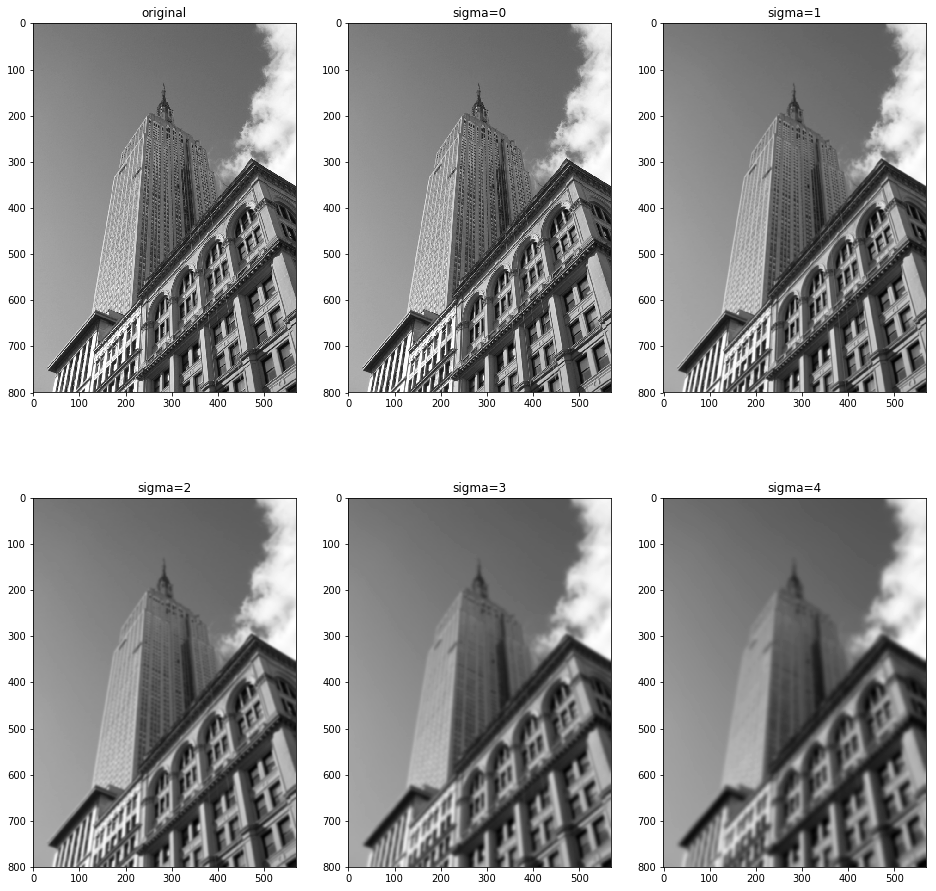
1.6.1 Take an image and apply Gaussian blur like in Figure 1.9. Plot the image contours for increasing values of sigma What happens? Can you explain why?

画像にガウシアンぼかしをかけろという問題。PILなどのライブラリーの使い方を覚えるためのものです。

私の回答

from PIL import Image
from numpy import *
from pylab import *
from scipy.ndimage import filters
from scipy import misc
import imtools

im = array(Image.open('data/empire.jpg').convert('L'))
figure(figsize=(16,16))
gray()
subplot(2, 3, 1)
title('original')
imshow(im)

for i in range(5):
    subplot(2, 3, i+2)
    title('sigma='+str(i))
    im1 = filters.gaussian_filter(im, i)
    imshow(im1)

show()

figure(figsize=(16,16))
gray()
subplot(2, 3, 1)
title('original')
imshow(im)

for i in range(5):
    subplot(2, 3, i+2)
    title('sigma='+str(i))
    im1 = filters.gaussian_filter(im, i)
    imx = zeros(im1.shape)
    filters.sobel(im1, 1, imx)
    imy = zeros(im1.shape)
    filters.sobel(im1, 0, imy)
    imxy = sqrt(imx**2+imy**2)
    imshow(imxy)

show()

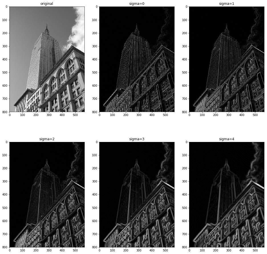
これは教科書のままですね。使用した画像は先ほどの著者の方のページからダウンロードできます
問題はぼかしだけでしたが、エッジ抽出もやってみました。

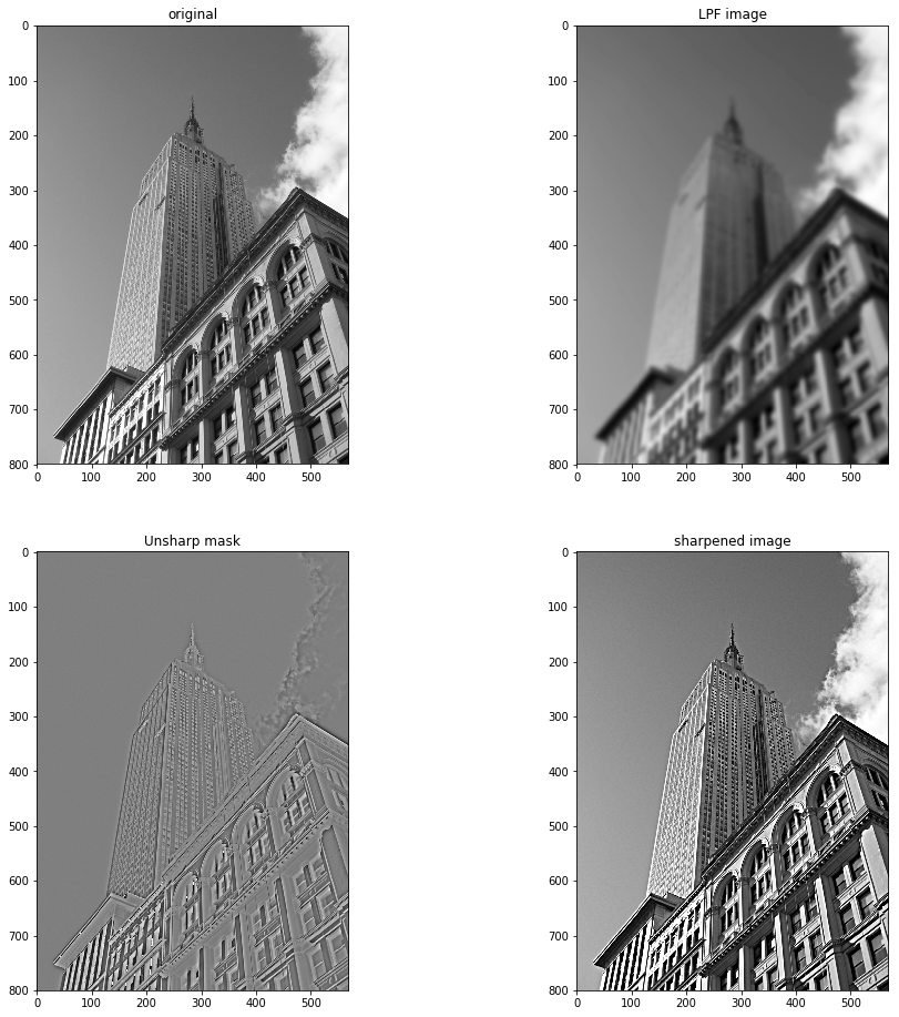
1.6.2 Implement an unsharp masking operation (http://en.wikipedia.org/wiki/Unsharp_masking) by blurring an image and then subtracting the blurred version from the original. This gives a sharpening effect to the image. Try this on both color and grayscale images.

第１問で作ったぼかし画像から原画像を引いてアンシャープマスクをかけろという問題。

私の回答

from PIL import Image
from numpy import *
from pylab import *
from scipy.ndimage import filters
from scipy import misc
import imtools

im = array(Image.open('data/empire.jpg').convert('L'))
im1 = zeros(im.shape)
im1 = filters.gaussian_filter(im, 4)
im2 = 1.0*im1-im
im3 = clip(im - 1*im2, 0, 255)

figure(figsize=(16, 16))
gray()
subplot(2, 2, 1)
title('original')
imshow(uint8(im))

subplot(2, 2, 2)
title('LPF image')
imshow(uint8(im1))

subplot(2, 2, 3)
title('Unsharp mask')
imshow(uint8(im2+128))

subplot(2, 2, 4)
title('sharpened image')
imshow(uint8(im3))

show()

im = array(Image.open('data/empire.jpg'))
im1 = zeros(im.shape)
for i in range(3):
    im1[:, :, i] = filters.gaussian_filter(im[:, :, i], 4)
im2 = 1.0*im1-im
im3 = uint8(clip(im - 1*im2, 0, 255))

figure(figsize=(16, 16))
subplot(2, 2, 1)
title('original')
imshow(im)

subplot(2, 2, 2)
title('LPF image')
imshow(uint8(im1))

subplot(2, 2, 3)
title('Unsharp mask')
imshow(uint8(im2))

subplot(2, 2, 4)
title('sharpened image')
imshow(im3)

show()

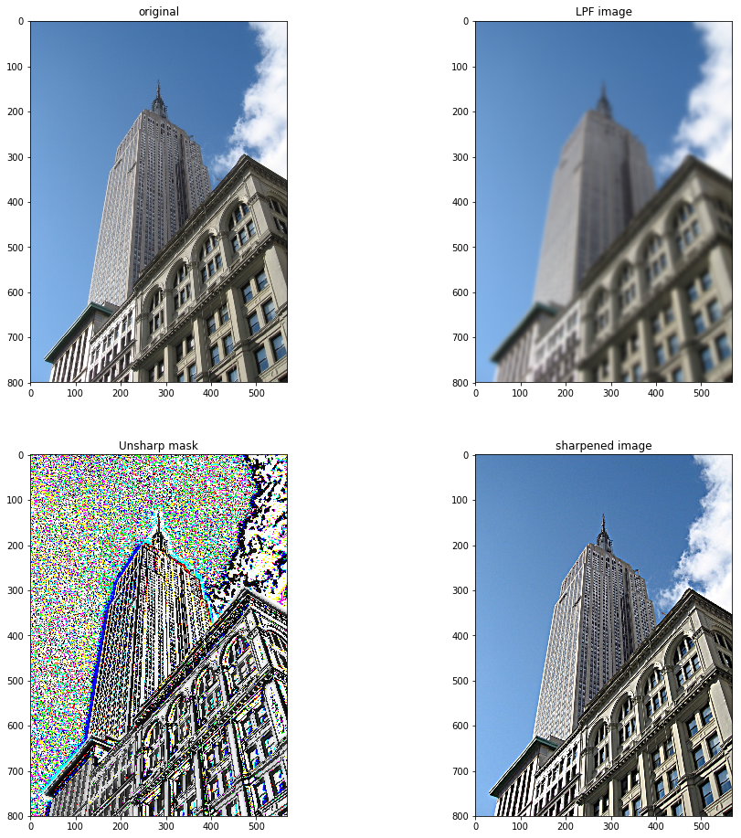
なんだかカラー版のアンシャープマスクが変な気がしますが、これはDC成分が抜いてあるので色情報が信用できないだけだと思います。鮮鋭化した画像はなおっています。

1.6.3 An alternative image normalization to histogram equalization is a quotient image.A quotient image is obtained by dividing the image with a blurred version I/(I*G). Implement this and try it on some sample images.

画像の正規化のために自己商画像をつくれという問題

私の回答

from PIL import Image
from numpy import *
from pylab import *
from scipy.ndimage import filters
from scipy import misc
import imtools

im = array(Image.open('data/empire.jpg').convert('L'))
im2, cdf = imtools.histeq(im)
im3 = 1.0*filters.gaussian_filter(im, 128)
im4 = clip(128 * (1.0 *im / (im3 + 0.1)), 0, 255)

figure(figsize=(16,16))
gray()
subplot(3, 2, 1)
title('original')
imshow(im)

subplot(3, 2, 2)
title('original hist')
hist(im.flatten(), 256, normed=True)

subplot(3, 2, 3)
gray()
title('histogram equalized')
imshow(im2)

subplot(3, 2, 4)
title('equalized hist')
hist(im2.flatten(), 256, normed=True)

subplot(3, 2, 5)
gray()
title('Self-quotient')
imshow(uint8(im4))

subplot(3, 2, 6)
title('Self-quantient quotient')
hist(im4.flatten(), 256, normed=True)

show()

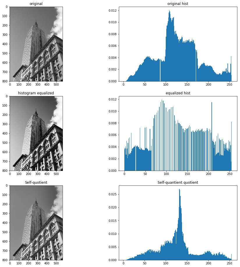
書いてあるとおりにやってみたのですが、これでいいのでしょうか。自己商画像はやったことがないのでわかりません。

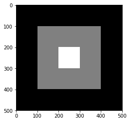
1.6.4 Write a function that finds the outline of simple objects in images (for example a square against white background) using image gradients.

画像の購買を使って輪郭を見つける関数を作れという問題
私の回答
https://github.com/moizumi99/CVBookExercise/blob/master/Chapter-1/CV%20Book%20Ch1%20Ex%204.ipynb

from numpy import *
from numpy import random
from scipy.ndimage import filters
from PIL import *
from pylab import *

im = zeros((500, 500))
im[100:400, 100:400] = 128
im[200:300, 200:300]=255
figure()
gray()
imshow(im)
show()

def edge(X, th):
    imx = zeros(X.shape)
    filters.sobel(X, 1, imx)
    imy = zeros(X.shape)
    filters.sobel(X, 0, imy)
    ims = sqrt(imx**2 + imy**2)
    ims[ims<th]=0
    ims[ims>=th]=1
    ims = uint8(ims)
    return ims

im2 = edge(im, 0.1)
figure()
gray()
imshow(im2)
show()

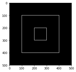
そのままです。scipy.ndimage.filtersのソーベルフィルターを使ってエッジ検出を行いました。

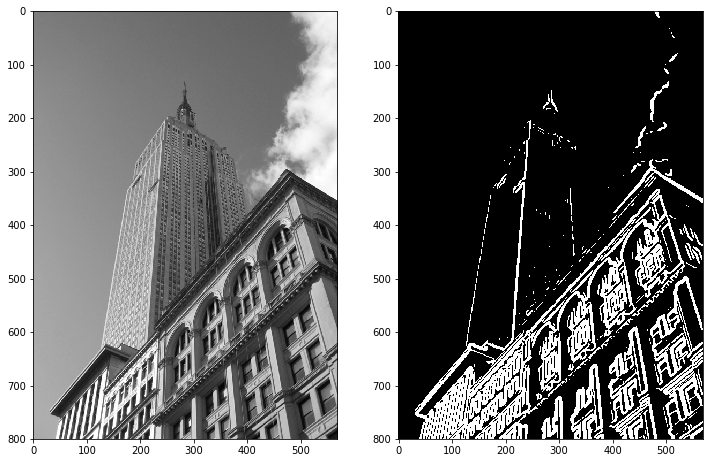
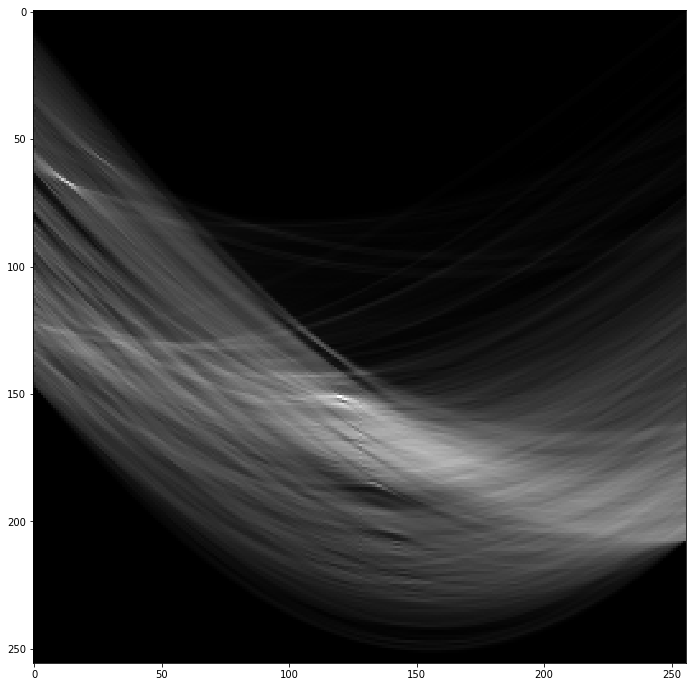
1.6.5 Use gradient direction and magnitude to detect lines in an image. Estimate the extent of the lines and their parameters. Plot the lines overlaid on the image.

勾配の強度と方向を使って線分を検出する問題。線分のパラメータを推定して線分を書けとも書いてあります。
前の問題までは教科書に書いてあるものだけですんだのですが、これはちょっと考えます。線分検出いえばハフ変換なのですが、ハフ変換のライブラリがどこにあるのかわかりません。ということで、ハフ変換をパイソンで実装してみました。

私の回答

from numpy import *
from numpy import random
from scipy.ndimage import filters
from PIL import *
from pylab import *

def edge(X, th):
    imx = zeros(X.shape)
    filters.gaussian_filter(X, (2,2), (0,1), imx)
    imy = zeros(X.shape)
    filters.gaussian_filter(X, (2,2), (1,0), imy)
    ims = sqrt(imx**2 + imy**2)
    ims[ims<th]=0
    ims[ims>=th]=1
    ims = uint8(ims)
    return ims

im2 = array(Image.open('data/empire.jpg').convert('L'))
im2e = edge(im2, 8)
figure(figsize=(12, 12))
gray()
subplot(1, 2, 1)
imshow(im2)
subplot(1, 2, 2)
imshow(im2e)
show()

# Hough transform
im3 = zeros((256, 256))
for y in range(im2e.shape[0]):
    for x in range(im2e.shape[1]):
        if (im2e[y, x]>0):
            for i in range(256):            
                t = math.pi/2*i/256
                r = x*math.cos(t)+y*sin(t)
                r = r*255/sqrt(im2e.shape[0]**2 + im2e.shape[1]**2)
                im3[int(r), i] = im3[int(r), i] + 1
figure(figsize=(12, 12))
gray()
imshow(im3)
show()

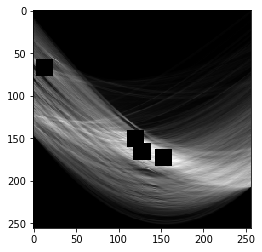
peaks=[]
im4 = np.array(im3)
for i in range(4):
    ym = argmax(im4)/im4.shape[0]
    xm = argmax(im4)%im4.shape[0]
    peaks.append([ym, xm])
    im4[ym-10:ym+10, xm-10:xm+10] = -1
print peaks
figure()
imshow(im4)
show()

[[151, 120], [67, 13], [166, 128], [173, 153]]

figure(figsize=(12, 12))
imshow(im4)
for [rmax, tmax] in peaks:
    rmax = 1.0*rmax
    tmax = 1.0*tmax
    print rmax, tmax
    im4 = im2.copy()
    t = math.pi/2*tmax/256
    r = rmax/256*math.sqrt(im2.shape[0]**2 + im2.shape[1]**2)
    print t, tmax/256*90, r, math.sqrt(im2.shape[0]**2 + im2.shape[1]**2)
    x0 = 0
    y0 = r/math.sin(t)
    if (y0<0):
        y0 = 0
        x0 = r/math.cos(t)
    elif (y0>=im4.shape[0]):
        y0 = im4.shape[0]
        x0 = (r-y0*math.sin(t))/math.cos(t)
    x1 = im4.shape[1]
    y1 = (r - math.cos(t)*x1)/math.sin(t)
    if (y1<0):
        y1 = 0
        x1 = r/math.cos(t)
    elif (y1>=im4.shape[0]):
        y1 = im4.shape[0]
        x1 = (r-y1*math.sin(t))/math.cos(t)
    plot([x0, x1], [y0, y1])
    print (x0, y0), (x1, y1)
show()

151.0 120.0
0.736310778185 42.1875 579.057453276 981.71329827
(56.427864089891706, 800) (569, 234.4637977246443)
67.0 13.0
0.0797670009701 4.5703125 256.932777282 981.71329827
(193.8030626400868, 800) (257.7523526199092, 0)
166.0 128.0
0.785398163397 45.0 636.579716847 981.71329827
(100.25966909651015, 800) (569, 331.25966909651004)
173.0 153.0
0.938796242186 53.7890625 663.423439846 981.71329827
(30.376813034067236, 800) (569, 405.62949971317215)

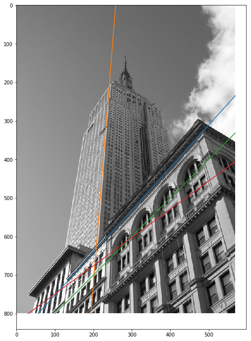
なんだかうまくいっているのか不安ですが、おそらくハフ変換にライブラリーを使えばもっと精度はよくなるのではないかと思います。第１０章のOpenCVの解説(10.5.3)でハフ変換がでてきます。

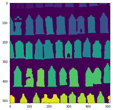
1.6.6 Apply the label() function to a thresholded image of your choice. Use histograms and the resulting label image to plot the distribution of object sizes in the image.

scipy.ndimage.measurements.label関数を閾値処理した画像に使大きさの分布をだしなさい、という問題。

私の回答

from numpy import *
from numpy import random
from scipy.ndimage import filters
from PIL import *
from pylab import *
from scipy.ndimage import measurements, morphology

im = array(Image.open('data/houses.png').convert('L'))
im = 1*(im<128)

labels, nbr_objects = measurements.label(im)
print "Number of objects", nbr_objects

figure(figsize=(6, 12))
imshow(labels)
show()

Number of objects 45

figure()
hist(labels.flatten())
axis([5, 45, 0, 20000])
show()

教科書と同じ家の画像を使いました。

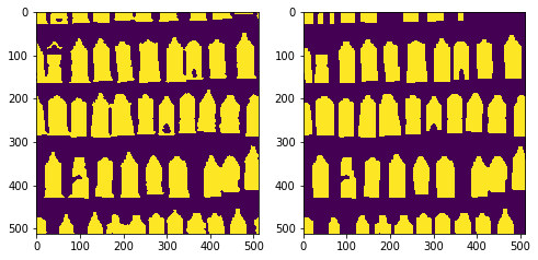
1.6.7 Experiment with successive morphological operations on a thresholded image of your choice. When you have found some settings that produce good results, try the function center_of_mass in morphology to find the center coordinates of each object and plot them in the image.

閾値処理した画像にモルフォロジー演算を用いて、最後に中心位置をみつけろという問題

私の回答

from numpy import *
from numpy import random
from scipy.ndimage import filters
from PIL import *
from pylab import *
from scipy.ndimage import measurements, morphology

im2 = array(Image.open('data/houses.png').convert('L'))
im2 = 1*(im2<64)
im_open = morphology.binary_opening(im2, ones((6, 3)), iterations=4)
figure(figsize=(8, 12))
subplot(1, 2, 1)
imshow(im2)
subplot(1, 2, 2)
imshow(im_open)
show()

labels2, nbr_objects2 = measurements.label(im_open)
print "Number of objects", nbr_objects2
center = measurements.center_of_mass(im_open, labels2, range(nbr_objects2))
figure(figsize=(8, 8))
imshow(im_open)
for i in range(nbr_objects2):
    plot(center[i][1], center[i][0], "*")
show()

Number of objects 47

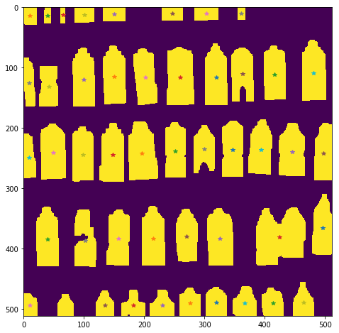
これでいいのかな？

１章終わり

まずは第１章終わりです。
ちょっと怪しい答えもありますが、だいたいできたと思います。まだチュートリアルですからね。