はじめに
Rで最適化問題を解くことができるらしいので,学部レベル(初級)のミクロ経済学の序盤で習う,「予算制約の中で効用(満足感)を最大化する購買量の探索」という効用最大化問題(最適消費計画問題)を例にとり,Rで簡単な制約付き最適化問題を解いたりイロイロしてみます。
◇2018年1月20日追記
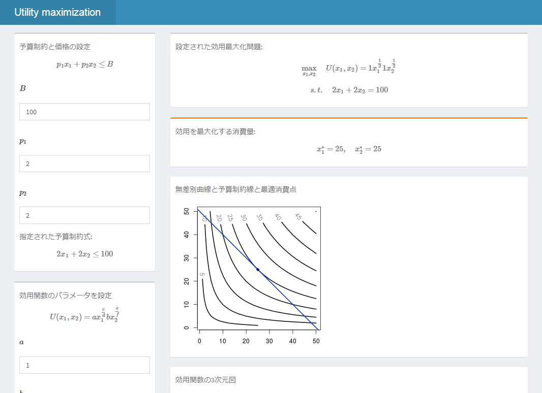
ここに載せたことをshinyで作動させてみました。
シンプルな効用最大化問題計算機という感じです。
https://nigimitama.shinyapps.io/MicroEconomics_01_UtilityMaximizationProblem/
中身のコードはこのページの下部(おまけ2)にあります。よろしければ御覧ください。
問題
2財モデルのこんな問題があるとします。
第1財の消費量を$x_1$,第2財の消費量を$x_2$と表す。ある家計の効用関数が$U(x_1,x_2)=x_1^{\frac{2}{5}}x_2^{\frac{3}{5}}$で表されるとする。予算が$100$,第1財の価格が$4$,第2財の価格が$6$のとき,効用を最大化する最適消費量はそれぞれいくらか?
$$\max_{x_1,x_2} \hspace{1em} x_1^{\frac{2}{5}}x_2^{\frac{3}{5}}$$
$$s.t. \hspace{1em} 100 = 4x_1+6x_2$$
ラグランジュの未定乗数法で解ける問題ですが,Rで解いてみます。
Rで解く
{Rsolnp}パッケージを使います。
library(Rsolnp)
ObjFunc = function(x) return( - x[1]^(2/5) * x[2]^(3/5) ) #目的関数
# solnp()は最小化をするようになっているので,目的関数にマイナスを掛ける

ConstFunc = function(x) return( x[1]* 4 + x[2] * 6 ) #制約式の右辺
eq.value <- c(100) #制約式の左辺

x0 <- c(1,1) #決定変数を初期化

solution <- solnp(x0, fun = ObjFunc, eqfun = ConstFunc, eqB = eq.value )
# 最適な「x_1」と「x_2」の値
solution$pars
[1] 10 10
最適な消費量$x_1^* , x_2^* $ は $x_1^* = 10, \ x_2^* = 10$であることが示された
(おまけ1)図示
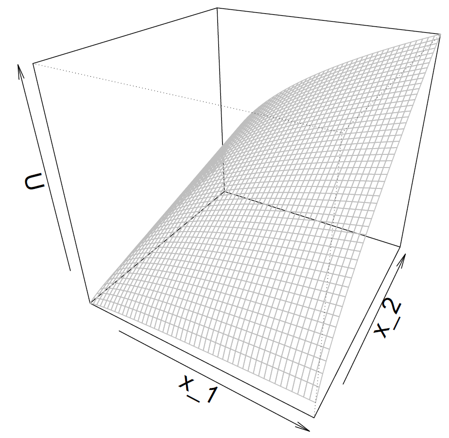
■効用関数の図示
モノ($x_1,x_2$)をたくさん買うほど効用$U$は上がる
# 3次元プロット:persp()
x_1 <- 1:50
x_2 <- 1:50
u <- function(x_1,x_2) {x_1^(2/5) * x_2^(3/5)} #効用関数を定義
U <- outer(x_1, x_2, u) #outer()はx_1,x_2に対応したf(x_1,x_2)の値を行列で返す
persp(x_1, x_2, U,
      theta = 30, # 横回転の角度
      phi = 30, # 縦回転の角度
      ticktype = "simple", # 線の種類
      lwd = 0.5, # 線の太さ
      col = F,
      border = 8)
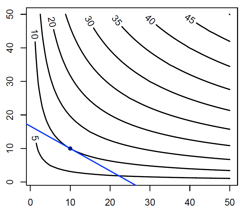
■等高線(無差別曲線)と予算制約線と最適消費点
効用関数の曲面を真上から見て等高線にした図。経済学ではこの等高線を無差別曲線という。
予算制約線(青い直線)と最適消費点(藍色の点)も記しておいた。
無差別曲線と予算制約線が接する点が最適消費点となる。
# 等高線:contour()
contour(x_1, x_2, U, method = "edge", labcex = 1,lwd = 2)
abline(a = 100/6, b = -4/6, lwd = 2, col = "blue") #予算制約線
points(x = 10, y = 10, lwd = 3, col = "darkblue", pch = 16) #最適消費点
(おまけ2)Shinyで効用最大化問題計算機を作る
以上の制約付き最適化問題を解く{Rsolnp}の処理や関数の図示などをshinyで行わせてみる。
# 日本語の文字列が本文中にあるとdeployできないみたい
# server側のRenderUI内の日本語は問題ないのでコレを利用

library(shinydashboard)
library(shiny)
library(Rsolnp)

header <- dashboardHeader(
  title = "Utility maximization problem"
)

body <- dashboardBody(
    column(width = 3,
           #予算制約
           box(width = NULL,
               uiOutput('budgettext'),
               numericInput("budget",
                            label = "$$B$$",
                            value = 100),
               numericInput("p_1",
                            label = "$$p_1$$",
                            value = 2),
               numericInput("p_2",
                            label = "$$p_2$$",
                            value = 2),
               uiOutput("budgetform")

           ),

           box(width = NULL,
               #効用関数モジュール
               uiOutput('utilityfunctiontext'),
               withMathJax(),   #TeX表記有効化
               numericInput("a",
                            label = "$$a$$",
                            value = 1),
               numericInput("b",
                            label = "$$b$$",
                            value = 1),
               numericInput("c",
                            label = "$$c$$",
                            value = 1),
               numericInput("d",
                            label = "$$d$$",
                            value = 2),
               numericInput("e",
                            label = "$$e$$",
                            value = 1),
               numericInput("f",
                            label = "$$f$$",
                            value = 2),
               uiOutput("utilityfunction")
               ),
           box(width = NULL,
               #p("変数の範囲(描画範囲)"),
               numericInput("range",
                            label =  "range of graph",
                            value = 50)
               )
    ),
    fluidRow(
      column(width = 7,
             #設定された効用最大化問題
             box(width = NULL,
                 uiOutput("Utilitymaximizationproblem")
             ),
             #効用最大化問題の解
             box(width = NULL, status = "warning",
                 uiOutput("maxutility")
                 ),
             #無差別曲線
             box(width = NULL, solidHeader = TRUE,
                 uiOutput('indifferencecurve'),
                 plotOutput("Plot2D", width = 300, height = 300)
                 ),
             box(width = NULL, solidHeader = TRUE,
                 uiOutput('Plot3Dtext'),
                 plotOutput("Plot3D",height = 300)
                 )
             )
      )
)

dashboardPage(
  header,
  dashboardSidebar(disable = TRUE),
  body
)
library(shinydashboard)
library(shiny)
library(Rsolnp)

# サーバロジックの定義
shinyServer(function(input, output) {

  # 予算制約式box見出し
  output$budgettext <- renderUI({
    withMathJax(helpText("予算制約と価格の設定$$p_1 x_1 + p_2 x_2 \\leq B$$"))
  })
  #指定された予算をTeXでUIに表示
  output$budgetform <- renderUI({
    withMathJax(helpText(paste0('指定された予算制約式:$$',
                                input$p_1,'x_1 + ', input$p_2,'x_2',
                                '\\leq',input$budget,'$$')))
  })


  # 効用関数box見出し
  output$utilityfunctiontext <- renderUI({
    withMathJax(helpText('効用関数のパラメータを設定$$U(x_1,x_2)=a x_1^ \\frac{c}{d} b x_2^ \\frac{e}{f}$$'))
  })
  #指定された効用関数をTeXでUIに表示
  output$utilityfunction <- renderUI({
    withMathJax(helpText(paste0('指定された効用関数:$$U(x_1,x_2)=',
                              input$a,'x_1','^\\frac{',input$c,'}','{',input$d,'}', input$b,'x_2','^\\frac{',input$e,'}','{',input$f,'}','$$')))
  })


  #設定された効用最大化問題
  output$Utilitymaximizationproblem <- renderUI({
    withMathJax(helpText(paste0(
      '設定された効用最大化問題:',

      '$$ \\max_{x_1,x_2} \\hspace{1em}  U(x_1,x_2)=',input$a,'x_1','^\\frac{',input$c,'}','{',input$d,'}', input$b,'x_2','^\\frac{',input$e,'}','{',input$f,'}$$',

      '$$s.t. \\hspace{1em} ', input$p_1,'x_1 + ', input$p_2,'x_2 \\leq',input$budget,'$$'
      )))
  })


  #最適消費計画の解
  output$maxutility <- renderUI({

    ObjFunc = function(x) return( - input$a * x[1]^(input$c/input$d) * input$b * x[2]^(input$e/input$f) ) #目的関数
    #solnp()は最小化をするようになっているので,目的関数にマイナスを掛ける
    ConstFunc = function(x) return( x[1]* input$p_1 + x[2] * input$p_2 ) #制約式の右辺
    eq.value <- c(input$budget) #制約式の左辺
    x0 <- c(1,1) #決定変数を初期化

    solution <- solnp(x0, fun = ObjFunc, eqfun = ConstFunc, eqB = eq.value )

    #return
    withMathJax(helpText(paste0("効用を最大化する消費量:",
                                '$$x_{1}^*=',solution$pars[1],', \\hspace{1em}  x_{2}^*=',solution$pars[2],'$$')))
  })


  #無差別曲線と予算制約線と最適消費点
  output$indifferencecurve <- renderUI({
    withMathJax(helpText('無差別曲線と予算制約線と最適消費点'))
  })
  output$Plot2D <- renderPlot({
    #以下のreactiveな要素をrenderPlotに入れれば使えるっぽい
    #効用関数をfunctionの形で定義
    u <- function(x_1,x_2) {input$a * x_1 ^ (input$c/input$d) * input$b * x_2 ^ (input$e/input$f)} #効用関数を定義

    #xの範囲指定
    x_1 <- 1:input$range
    x_2 <- 1:input$range
    U <- outer(x_1, x_2, u) #outer()はx_1,x_2に対応したf(x_1,x_2)の値を行列で返す

    #plot
    par(mar=c(3,3,1,1))
    contour(x_1, x_2, U, method = "edge", labcex = 1,lwd = 2)
    abline(a = input$budget/input$p_2, b = -input$p_1/input$p_2, lwd = 2, col = "blue") #予算制約線 x_2 = ...

    #最適消費点
    ObjFunc = function(x) return( - input$a * x[1]^(input$c/input$d) * input$b * x[2]^(input$e/input$f) ) #目的関数
    #solnp()は最小化をするようになっているので,目的関数にマイナスを掛ける
    ConstFunc = function(x) return( x[1]* input$p_1 + x[2] * input$p_2 ) #制約式の右辺
    eq.value <- c(input$budget) #制約式の左辺
    x0 <- c(1,1) #決定変数を初期化
    solution <- solnp(x0, fun = ObjFunc, eqfun = ConstFunc, eqB = eq.value )
    points(x = solution$pars[1], y = solution$pars[2], lwd = 3, col = "darkblue", pch = 16) #最適消費点

  })

  #3D plot of utility function 効用関数の3次元図
  output$Plot3Dtext <- renderUI({
    withMathJax(helpText('効用関数の3次元図'))
  })
  output$Plot3D <- renderPlot({

    #以下のreactiveな要素をrenderPlotに入れれば使えるっぽい
    #効用関数をfunctionの形で定義
    u <- function(x_1,x_2) {input$a * x_1 ^ (input$c/input$d) * input$b * x_2 ^ (input$e/input$f)} #効用関数を定義

    #xの範囲指定
    x_1 <- 1:input$range
    x_2 <- 1:input$range
    U <- outer(x_1, x_2, u) #outer()はx_1,x_2に対応したf(x_1,x_2)の値を行列で返す
    persp(x_1, x_2, U,
          theta = 30, # 横回転の角度。ここをいじって表示のアングルを変える。
          phi = 20, # 縦回転の角度。ここをいじって表示のアングルを変える。
          ticktype = "simple", # 線の種類
          lwd = 0.5, # 線が太いと見づらかったりするので0.5にしておいた。
          col = F, #塗りつぶしなし
          border = 8 #枠線灰色
          )
  })
})