学習済みのCNNモデルを用いて猫画像と犬画像を分類する方法の紹介 Part3
前回は、データ拡張を用いて訓練データを増やして学習済みモデルに訓練をさせました。※前回の記事
今回は上記に加えさらに、訓練済みのモデルの一部のみを本データにより再訓練を行うことで最適化させることでより精度の高いモデルの作成を試みます。
モデルの読み込み
from keras.applications import VGG16

# 学習済モデル VGG16のインスタンスを生成
conv_base = VGG16(
    weights = 'imagenet', # 重みのチェックポイント箇所
    include_top = False,  # 全結合分類器を含めるかどうか(元のモデルは1000個のラベルに分類するモデル)
    input_shape = (150, 150, 3) # 画像テンソルの形状(省略した場合はネットワークが任意に判断)
)

conv_base.summary()

Layer (type)                 Output Shape              Param #
=================================================================
input_1 (InputLayer)         (None, 150, 150, 3)       0
_________________________________________________________________
block1_conv1 (Conv2D)        (None, 150, 150, 64)      1792
_________________________________________________________________
block1_conv2 (Conv2D)        (None, 150, 150, 64)      36928
_________________________________________________________________
block1_pool (MaxPooling2D)   (None, 75, 75, 64)        0
_________________________________________________________________
block2_conv1 (Conv2D)        (None, 75, 75, 128)       73856
_________________________________________________________________
block2_conv2 (Conv2D)        (None, 75, 75, 128)       147584
_________________________________________________________________
block2_pool (MaxPooling2D)   (None, 37, 37, 128)       0
_________________________________________________________________
block3_conv1 (Conv2D)        (None, 37, 37, 256)       295168
_________________________________________________________________
block3_conv2 (Conv2D)        (None, 37, 37, 256)       590080
_________________________________________________________________
block3_conv3 (Conv2D)        (None, 37, 37, 256)       590080
_________________________________________________________________
block3_pool (MaxPooling2D)   (None, 18, 18, 256)       0
_________________________________________________________________
block4_conv1 (Conv2D)        (None, 18, 18, 512)       1180160
_________________________________________________________________
block4_conv2 (Conv2D)        (None, 18, 18, 512)       2359808
_________________________________________________________________
block4_conv3 (Conv2D)        (None, 18, 18, 512)       2359808
_________________________________________________________________
block4_pool (MaxPooling2D)   (None, 9, 9, 512)         0
_________________________________________________________________
block5_conv1 (Conv2D)        (None, 9, 9, 512)         2359808
_________________________________________________________________
block5_conv2 (Conv2D)        (None, 9, 9, 512)         2359808
_________________________________________________________________
block5_conv3 (Conv2D)        (None, 9, 9, 512)         2359808
_________________________________________________________________
block5_pool (MaxPooling2D)   (None, 4, 4, 512)         0
=================================================================
Total params: 14,714,688
Trainable params: 14,714,688
Non-trainable params: 0
_________________________________________________________________
画像を用意
なお、オリジナルデータはKaggleのサイトからダウンロードしてます。
詳しくは只今勉強中!学習済みモデルを用いた機械学習 画像分類を参照してください。
# 訓練画像を用意
import os, shutil
"""
データの準備
"""

# オリジナルデータ
original_dataset_dir = 'C:\\Users\\minarai\\Downloads\\dogs-vs-cats\\train'

# 縮小画像を格納するディレクトリ
base_dir = 'C:\\Users\\minarai\\Pictures\\dogs-vs-cats\\base_dir'
if os.path.isdir(base_dir) == False:
    os.mkdir(base_dir)

# 訓練データ、検証データ、テストデータ用のディレクトリ
train_dir      = os.path.join(base_dir, 'train')
validation_dir = os.path.join(base_dir, 'validation')
test_dir       = os.path.join(base_dir, 'test')
if os.path.isdir(train_dir) == False:
    os.mkdir(train_dir)
if os.path.isdir(validation_dir) == False:
    os.mkdir(validation_dir)
if os.path.isdir(test_dir) == False:
    os.mkdir(test_dir)

# 訓練用 犬、猫のディレクトリ
train_dogs_dir = os.path.join(train_dir, 'dogs')
train_cats_dir = os.path.join(train_dir, 'cats')
if os.path.isdir(train_dogs_dir) == False:
    os.mkdir(train_dogs_dir)
if os.path.isdir(train_cats_dir) == False:
    os.mkdir(train_cats_dir)

# 検証用 犬、猫のディレクトリ
validation_dogs_dir = os.path.join(validation_dir, 'dogs')
validation_cats_dir = os.path.join(validation_dir, 'cats')
if os.path.isdir(validation_dogs_dir) == False:
    os.mkdir(validation_dogs_dir)
if os.path.isdir(validation_cats_dir) == False:
    os.mkdir(validation_cats_dir)

# テスト用 犬、猫のディレクトリ
test_dogs_dir = os.path.join(test_dir, 'dogs')
test_cats_dir = os.path.join(test_dir, 'cats')
if os.path.isdir(test_dogs_dir) == False:
    os.mkdir(test_dogs_dir)
if os.path.isdir(test_cats_dir) == False:
    os.mkdir(test_cats_dir)

# 訓練用データをコピー ※画像名は cat.i.jpg/dog.i.jpg 格納されている
for i in range(2000):
    cat_file = 'cat.{}.jpg'.format(i)
    dog_file = 'dog.{}.jpg'.format(i)

    cat_src = os.path.join(original_dataset_dir, cat_file)
    dog_src = os.path.join(original_dataset_dir, dog_file)
    if i < 1000:
        cat_dst = os.path.join(train_cats_dir, cat_file)
        shutil.copyfile(cat_src, cat_dst)

        dog_dst = os.path.join(train_dogs_dir, dog_file)
        shutil.copyfile(dog_src, dog_dst)
    elif i < 1500:
        cat_dst = os.path.join(validation_cats_dir, cat_file)
        shutil.copyfile(cat_src, cat_dst)

        dog_dst = os.path.join(validation_dogs_dir, dog_file)
        shutil.copyfile(dog_src, dog_dst)
    else:
        cat_dst = os.path.join(test_cats_dir, cat_file)
        shutil.copyfile(cat_src, cat_dst)

        dog_dst = os.path.join(test_dogs_dir, dog_file)
        shutil.copyfile(dog_src, dog_dst)

print('total training cat images:', len(os.listdir(train_cats_dir)))
print('total training dog images:', len(os.listdir(train_dogs_dir)))

print('total validation cat images:', len(os.listdir(validation_cats_dir)))
print('total validation dog  images:', len(os.listdir(validation_dogs_dir)))

print('total test cat images:', len(os.listdir(test_cats_dir)))
print('total test dog images:', len(os.listdir(test_dogs_dir)))

# データを表示
total training cat images: 1000
total training dog images: 1000
total validation cat images: 500
total validation dog images: 500
total test cat images: 500
total test dog images: 500
モデル定義
学習済みのモデルに全結合分類器層と2値分類層を追加します。
# 全結合分類器の定義
from keras import layers
from keras import models
from keras import optimizers

# モデルに学習済みモデルを追加後、分類器を追加していく
model = models.Sequential()
model.add(conv_base)
model.add(layers.Flatten())
model.add(layers.Dense(256, activation='relu')) # 200万個のパラメータから分類している
model.add(layers.Dense(1, activation='sigmoid'))

model.summary()

"""
学習済みモデルの重みを凍結しておくことで、学習済みモデルのモデルの重みは更新(破壊)せずに新たに追加したモデルに対して訓練をさせることができる
"""
print('This is the number of trainable weights brefore freezing the conv_base:', len(model.trainable_weights))
conv_base.trainable = False

print('This is the number of trainable weights after freezing the conv_base:', len(model.trainable_weights))

Layer (type)                 Output Shape              Param #
=================================================================
vgg16 (Model)                (None, 4, 4, 512)         14714688
_________________________________________________________________
flatten_1 (Flatten)          (None, 8192)              0
_________________________________________________________________
dense_1 (Dense)              (None, 256)               2097408
_________________________________________________________________
dense_2 (Dense)              (None, 1)                 257
=================================================================
Total params: 16,812,353
Trainable params: 16,812,353
Non-trainable params: 0
_________________________________________________________________
This is the number of trainable weights brefore freezing the conv_base: 30
This is the number of trainable weights after freezing the conv_base: 4
データの前処理
前回同様、訓練データを拡張(水増し)します。
※検証データは拡張しません。
# 訓練データ、検証データの作成
from keras.preprocessing import image
import matplotlib.pyplot as plt
from keras.preprocessing.image import ImageDataGenerator

# データ拡張の実践例
train_datagen = ImageDataGenerator(
    rescale             = 1./255,   # 画像を再スケーリング
    rotation_range      = 40,       # 画像をランダムに回転させる範囲(0 - 180)
    width_shift_range   = 0.2,      # 切り取り位置をランダムに移動させる範囲
    height_shift_range  = 0.2,      # 切り取り位置をランダムに移動させる範囲
    shear_range         = 0.2,      # 等積変形をランダムに適用
    zoom_range          = 0.2,      # 描画内をランダムにズーム
    horizontal_flip     = True,     # 画像の半分を水平線方向にランダムに反転
    fill_mode           = 'nearest' # 描画範囲がオリジナルデータ外の場合の描画方法
)

# テストデータと検証データは拡張させない!
test_datagen = ImageDataGenerator(rescale = 1./255)

# flow_from_directory() : 指定したディレクトリ配下のファイルを生成する関数
train_generator = train_datagen.flow_from_directory(
    train_dir, # 対象画像パス
    target_size = (150, 150),
    batch_size  = 32,
    class_mode  = 'binary'
)

validation_generator = test_datagen.flow_from_directory(
    validation_dir, # 対象画像パス
    target_size = (150, 150),
    batch_size  = 32,
    class_mode  = 'binary'
)

Found 2000 images belonging to 2 classes.
Found 1000 images belonging to 2 classes.
モデルのファインチューニング
※model.trainableプロパティはBoolean値を取ります。
Falseの場合、モデルは凍結されますが、Trueの時、訓練データによってモデルは再訓練されます。
下記の例ではblock5_conv1層の時にtrainableの値をTrueにセットし、モデルを再訓練させるようにするようにしています。
# ファインチューニングする層を選択
conv_base.trainable = True

# モデル訓練凍結フラグ
set_trainable = False
for layer in conv_base.layers:
    if layer.name == 'block5_conv1':
        set_trainable = True
    else:
        set_trainable = False
    if set_trainable == True:
        layer.trainable = True
    else:
        layer.trainable = False

# モデルのファインチューニング
model.compile(loss='binary_crossentropy', optimizer=optimizers.RMSprop(lr=1e-5), metrics=['acc'])

history = model.fit_generator(
    train_generator,
    steps_per_epoch=100,
    epochs=100,
    validation_data=validation_generator,
    validation_steps=50
)
訓練結果を表示
%matplotlib inline
# 訓練データをプロット
import matplotlib.pyplot as plt
acc = history.history['acc']
val_acc = history.history['val_acc']
loss = history.history['loss']
val_loss = history.history['val_loss']
epochs = range(1, len(acc) + 1)
# スムーズにプロットされるように改良
def smooth_curve(points, factor=0.8):
smoothed_points = []
for point in points:
if smoothed_points:
previous = smoothed_points[-1]
smoothed_points.append(previous * factor + point * (1 - factor))
else:
smoothed_points.append(point)
return smoothed_points
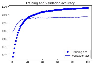
# 正解率
plt.plot(epochs, smooth_curve(acc), 'bo', label='Training acc')
plt.plot(epochs, smooth_curve(val_acc), 'b', label='Validation acc')
plt.title('Training and Validation accuracy')
plt.legend()
plt.figure()
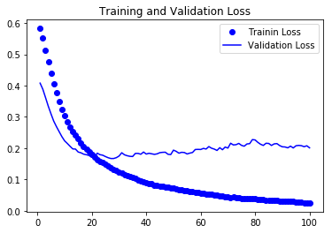
# 損失値
plt.plot(epochs, smooth_curve(loss), 'bo', label='Trainin Loss')
plt.plot(epochs, smooth_curve(val_loss), 'b', label='Validation Loss')
plt.title('Training and Validation Loss')
plt.legend()
plt.figure()
plt.show()
正解率と損失値のグラフを描画
まとめ
前回のグラフと今回のグラフを比較すると一目瞭然です。
ファインチューニングを行った結果、正解率は99%を超えました。
(グラフではわかりにくいのですが、検証データで99.12%でした。)
また、損失値も0.1%を切っており、素晴らしい結果が出ていますね。
ちなみに、今回の演習ではドロップアウト層を追加していませんが、ドロップアウト層を追加することによってより効率的なモデルの訓練を行う可能性もあります。
出来過ぎな気がしますが、演習としては良い結果が出てよかったです!