線形回帰を本当はPythonで解きたいけど表計算で解けと言われたので と 線形重回帰を本当はPythonで解きたいけど表計算で解けと言われたので の続編です。前の記事を読んでもらっていれば、曲線に回帰するのは簡単。
用いるデータ
import pandas as pd
data = [['HF', 19.5, 20.0],
        ['HCl', -84.9, 36.5],
        ['HBr', -67.0, 80.9],
        ['HI', -35.1, 127.9],
        ['H2O', 100.0, 18.0],
        ['H2S', -60.7, 34.1],
        ['H2Se', -42, 81.0],
        ['H2Te', -1.8, 129.6],
        ['NH3', -33.4, 17.0],
        ['PH3', -87, 34.0],
        ['AsH3', -55, 77.9],
        ['SbH3', -17.1, 124.8],
        ['CH4', -161.49, 16.0],
        ['SiH4', -111.8, 32.1],
        ['GeH4', -90, 76.6],
        ['SnH4', -52, 122.7],
        ['He', -268.934, 4.0],
        ['Ne', -246.048, 20.2],
        ['Ar', -185.7, 39.9],
        ['Kr', -152.3, 83.8],
        ['Xe', -108.1, 131.3],
       ]
df = pd.DataFrame(data, columns = ['molecule', 'boiling point', 'molecular weight'])
df
| molecule | boiling point | molecular weight | |
|---|---|---|---|
| 0 | HF | 19.500 | 20.0 |
| 1 | HCl | -84.900 | 36.5 |
| 2 | HBr | -67.000 | 80.9 |
| 3 | HI | -35.100 | 127.9 |
| 4 | H2O | 100.000 | 18.0 |
| 5 | H2S | -60.700 | 34.1 |
| 6 | H2Se | -42.000 | 81.0 |
| 7 | H2Te | -1.800 | 129.6 |
| 8 | NH3 | -33.400 | 17.0 |
| 9 | PH3 | -87.000 | 34.0 |
| 10 | AsH3 | -55.000 | 77.9 |
| 11 | SbH3 | -17.100 | 124.8 |
| 12 | CH4 | -161.490 | 16.0 |
| 13 | SiH4 | -111.800 | 32.1 |
| 14 | GeH4 | -90.000 | 76.6 |
| 15 | SnH4 | -52.000 | 122.7 |
| 16 | He | -268.934 | 4.0 |
| 17 | Ne | -246.048 | 20.2 |
| 18 | Ar | -185.700 | 39.9 |
| 19 | Kr | -152.300 | 83.8 |
| 20 | Xe | -108.100 | 131.3 |
X = df.loc[:, ['molecular weight']].as_matrix()
X
array([[  20. ],
       [  36.5],
       [  80.9],
       [ 127.9],
       [  18. ],
       [  34.1],
       [  81. ],
       [ 129.6],
       [  17. ],
       [  34. ],
       [  77.9],
       [ 124.8],
       [  16. ],
       [  32.1],
       [  76.6],
       [ 122.7],
       [   4. ],
       [  20.2],
       [  39.9],
       [  83.8],
       [ 131.3]])
Y = df['boiling point'].as_matrix()
Y
array([  19.5  ,  -84.9  ,  -67.   ,  -35.1  ,  100.   ,  -60.7  ,
        -42.   ,   -1.8  ,  -33.4  ,  -87.   ,  -55.   ,  -17.1  ,
       -161.49 , -111.8  ,  -90.   ,  -52.   , -268.934, -246.048,
       -185.7  , -152.3  , -108.1  ])
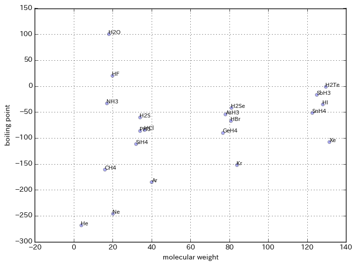
%matplotlib inline
import matplotlib.pyplot as plt
# 散布図
plt.figure(figsize=(8,6))
plt.scatter(X, Y, alpha=0.3)
for name, x, y in zip(df.loc[:, ['molecule']].as_matrix(), X, Y):
    plt.text(x, y, name[0], size=8)
plt.xlabel('molecular weight')
plt.ylabel('boiling point')
plt.grid()
plt.show()
import math
import numpy as np
logX = np.array([[math.log(x)] for x in X[:,0]])
logX
array([[ 2.99573227],
       [ 3.59731226],
       [ 4.39321382],
       [ 4.85124871],
       [ 2.89037176],
       [ 3.52929738],
       [ 4.39444915],
       [ 4.86445278],
       [ 2.83321334],
       [ 3.52636052],
       [ 4.35542595],
       [ 4.82671246],
       [ 2.77258872],
       [ 3.46885603],
       [ 4.33859708],
       [ 4.80974235],
       [ 1.38629436],
       [ 3.0056826 ],
       [ 3.68637632],
       [ 4.42843301],
       [ 4.87748478]])
まずは一番便利な scikit-learn から
from sklearn import linear_model
lr = linear_model.LinearRegression()
lr.fit(logX, Y)
LinearRegression(copy_X=True, fit_intercept=True, n_jobs=1, normalize=False)
# 回帰係数
lr.coef_
array([ 33.87205496])
# 切片
lr.intercept_
-211.66384118386563
print("y = f(x) = wlogx + t; (w, t) = ({0}, {1})".format(lr.coef_[0], lr.intercept_))
y = f(x) = wlogx + t; (w, t) = (33.872054963641745, -211.66384118386563)
# 決定係数R2
lr.score(logX, Y)
0.13487033631665779
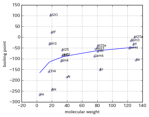
%matplotlib inline
import matplotlib.pyplot as plt
# 散布図
plt.figure(figsize=(5,4))
plt.scatter(X, Y, alpha=0.3)

# 回帰直線
plt.plot(sorted(X), sorted(lr.predict(logX)))
for name, x, y in zip(df.loc[:, ['molecule']].as_matrix(), X, Y):
    plt.text(x, y, name[0], size=8)
plt.xlabel('molecular weight')
plt.ylabel('boiling point')
plt.grid()
plt.show()
次は、ガチPythonで。
# 平均値を求める関数
def mean(list):
    sum = 0
    for x in list:
        sum += x
    return sum / len(list)
# 分散を求める関数
def variance(list):
    ave = mean(list)
    sum = 0
    for x in list:
        sum += (x - ave) ** 2
    return sum / len(list)
# 標準偏差を求める関数
import math
def standard_deviation(list):
    return math.sqrt(variance(list))
# 共分散 = 偏差積の平均
def covariance(list1, list2):
    mean1 = mean(list1)
    mean2 = mean(list2)
    sum = 0
    for d1, d2 in zip(list1, list2):
        sum += (d1 - mean1) * (d2 - mean2)
    return sum / len(list1)
# 相関係数 = 共分散を list1, list2 の標準偏差で割ったもの
def correlation(list1, list2):
    return covariance(list1, list2) / (standard_deviation(list1) * standard_deviation(list2))
# 回帰直線の傾き=相関係数*((yの標準偏差)/(xの標準偏差))
def w_fit(xlist, ylist):
    return correlation(xlist, ylist) * standard_deviation(ylist) / standard_deviation(xlist)
# y切片=yの平均-(傾き*xの平均)
def t_fit(xlist, ylist):
    return mean(ylist) - w_fit(xlist, ylist) * mean(xlist)
# 回帰直線の式を表示
w = w_fit(logX, Y)
t = t_fit(logX, Y)
print("y = f(x) = wlogx + t; (w, t) = ({0}, {1})".format(w, t))
y = f(x) = wlogx + t; (w, t) = ([ 33.87205496], [-211.66384118])
# 回帰直線の式を関数として表現
def f(x):
    return w * x + t
# 決定係数R2
def r2(xlist, ylist):
    wa1 = 0.
    wa2 = 0.
    for x, y in zip(xlist, ylist):
        wa1 += (y - f(x))**2
        wa2 += (y - mean(ylist))**2
    return 1. - wa1 / wa2
r2(logX, Y)
array([ 0.13487034])
さて、表計算で解けと言われたので pandas で書いてみましょうか。
import copy
from IPython.display import display
excel = copy.deepcopy(df)
excel
| molecule | boiling point | molecular weight | |
|---|---|---|---|
| 0 | HF | 19.500 | 20.0 |
| 1 | HCl | -84.900 | 36.5 |
| 2 | HBr | -67.000 | 80.9 |
| 3 | HI | -35.100 | 127.9 |
| 4 | H2O | 100.000 | 18.0 |
| 5 | H2S | -60.700 | 34.1 |
| 6 | H2Se | -42.000 | 81.0 |
| 7 | H2Te | -1.800 | 129.6 |
| 8 | NH3 | -33.400 | 17.0 |
| 9 | PH3 | -87.000 | 34.0 |
| 10 | AsH3 | -55.000 | 77.9 |
| 11 | SbH3 | -17.100 | 124.8 |
| 12 | CH4 | -161.490 | 16.0 |
| 13 | SiH4 | -111.800 | 32.1 |
| 14 | GeH4 | -90.000 | 76.6 |
| 15 | SnH4 | -52.000 | 122.7 |
| 16 | He | -268.934 | 4.0 |
| 17 | Ne | -246.048 | 20.2 |
| 18 | Ar | -185.700 | 39.9 |
| 19 | Kr | -152.300 | 83.8 |
| 20 | Xe | -108.100 | 131.3 |
excel['y'] = excel['boiling point']
excel['x'] = excel['molecular weight']
excel['log(x)'] = [math.log(x) for x in excel['x']]
mean_y = mean(excel['y'])
mean_logx = mean(excel['log(x)'])
display(excel, pd.DataFrame([[mean_y, mean_logx]], columns=['y','log(x)'], index=['mean']))
| molecule | boiling point | molecular weight | y | x | log(x) | |
|---|---|---|---|---|---|---|
| 0 | HF | 19.500 | 20.0 | 19.500 | 20.0 | 2.995732 |
| 1 | HCl | -84.900 | 36.5 | -84.900 | 36.5 | 3.597312 |
| 2 | HBr | -67.000 | 80.9 | -67.000 | 80.9 | 4.393214 |
| 3 | HI | -35.100 | 127.9 | -35.100 | 127.9 | 4.851249 |
| 4 | H2O | 100.000 | 18.0 | 100.000 | 18.0 | 2.890372 |
| 5 | H2S | -60.700 | 34.1 | -60.700 | 34.1 | 3.529297 |
| 6 | H2Se | -42.000 | 81.0 | -42.000 | 81.0 | 4.394449 |
| 7 | H2Te | -1.800 | 129.6 | -1.800 | 129.6 | 4.864453 |
| 8 | NH3 | -33.400 | 17.0 | -33.400 | 17.0 | 2.833213 |
| 9 | PH3 | -87.000 | 34.0 | -87.000 | 34.0 | 3.526361 |
| 10 | AsH3 | -55.000 | 77.9 | -55.000 | 77.9 | 4.355426 |
| 11 | SbH3 | -17.100 | 124.8 | -17.100 | 124.8 | 4.826712 |
| 12 | CH4 | -161.490 | 16.0 | -161.490 | 16.0 | 2.772589 |
| 13 | SiH4 | -111.800 | 32.1 | -111.800 | 32.1 | 3.468856 |
| 14 | GeH4 | -90.000 | 76.6 | -90.000 | 76.6 | 4.338597 |
| 15 | SnH4 | -52.000 | 122.7 | -52.000 | 122.7 | 4.809742 |
| 16 | He | -268.934 | 4.0 | -268.934 | 4.0 | 1.386294 |
| 17 | Ne | -246.048 | 20.2 | -246.048 | 20.2 | 3.005683 |
| 18 | Ar | -185.700 | 39.9 | -185.700 | 39.9 | 3.686376 |
| 19 | Kr | -152.300 | 83.8 | -152.300 | 83.8 | 4.428433 |
| 20 | Xe | -108.100 | 131.3 | -108.100 | 131.3 | 4.877485 |
| y | log(x) | |
|---|---|---|
| mean | -82.898667 | 3.801516 |
excel['y-mean(y)'] = [y - mean_y for y in excel['y']]
excel['log(x)-mean(log(x))'] = [logx - mean_logx for logx in excel['log(x)']]
display(excel, pd.DataFrame([[mean_y, mean_logx]], columns=['y','log(x)'], index=['mean']))
| molecule | boiling point | molecular weight | y | x | log(x) | y-mean(y) | log(x)-mean(log(x)) | |
|---|---|---|---|---|---|---|---|---|
| 0 | HF | 19.500 | 20.0 | 19.500 | 20.0 | 2.995732 | 102.398667 | -0.805784 |
| 1 | HCl | -84.900 | 36.5 | -84.900 | 36.5 | 3.597312 | -2.001333 | -0.204204 |
| 2 | HBr | -67.000 | 80.9 | -67.000 | 80.9 | 4.393214 | 15.898667 | 0.591697 |
| 3 | HI | -35.100 | 127.9 | -35.100 | 127.9 | 4.851249 | 47.798667 | 1.049732 |
| 4 | H2O | 100.000 | 18.0 | 100.000 | 18.0 | 2.890372 | 182.898667 | -0.911145 |
| 5 | H2S | -60.700 | 34.1 | -60.700 | 34.1 | 3.529297 | 22.198667 | -0.272219 |
| 6 | H2Se | -42.000 | 81.0 | -42.000 | 81.0 | 4.394449 | 40.898667 | 0.592933 |
| 7 | H2Te | -1.800 | 129.6 | -1.800 | 129.6 | 4.864453 | 81.098667 | 1.062936 |
| 8 | NH3 | -33.400 | 17.0 | -33.400 | 17.0 | 2.833213 | 49.498667 | -0.968303 |
| 9 | PH3 | -87.000 | 34.0 | -87.000 | 34.0 | 3.526361 | -4.101333 | -0.275156 |
| 10 | AsH3 | -55.000 | 77.9 | -55.000 | 77.9 | 4.355426 | 27.898667 | 0.553909 |
| 11 | SbH3 | -17.100 | 124.8 | -17.100 | 124.8 | 4.826712 | 65.798667 | 1.025196 |
| 12 | CH4 | -161.490 | 16.0 | -161.490 | 16.0 | 2.772589 | -78.591333 | -1.028928 |
| 13 | SiH4 | -111.800 | 32.1 | -111.800 | 32.1 | 3.468856 | -28.901333 | -0.332660 |
| 14 | GeH4 | -90.000 | 76.6 | -90.000 | 76.6 | 4.338597 | -7.101333 | 0.537081 |
| 15 | SnH4 | -52.000 | 122.7 | -52.000 | 122.7 | 4.809742 | 30.898667 | 1.008226 |
| 16 | He | -268.934 | 4.0 | -268.934 | 4.0 | 1.386294 | -186.035333 | -2.415222 |
| 17 | Ne | -246.048 | 20.2 | -246.048 | 20.2 | 3.005683 | -163.149333 | -0.795834 |
| 18 | Ar | -185.700 | 39.9 | -185.700 | 39.9 | 3.686376 | -102.801333 | -0.115140 |
| 19 | Kr | -152.300 | 83.8 | -152.300 | 83.8 | 4.428433 | -69.401333 | 0.626917 |
| 20 | Xe | -108.100 | 131.3 | -108.100 | 131.3 | 4.877485 | -25.201333 | 1.075968 |
| y | log(x) | |
|---|---|---|
| mean | -82.898667 | 3.801516 |
excel['(y-mean(y))**2'] = [sa ** 2 for sa in excel['y-mean(y)']]
excel['(log(x)-mean(log(x)))**2'] = [sa ** 2 for sa in excel['log(x)-mean(log(x))']]
display(excel, pd.DataFrame([[mean_y, mean_logx]], columns=['y','log(x)'], index=['mean']))
| molecule | boiling point | molecular weight | y | x | log(x) | y-mean(y) | log(x)-mean(log(x)) | (y-mean(y))**2 | (log(x)-mean(log(x)))**2 | |
|---|---|---|---|---|---|---|---|---|---|---|
| 0 | HF | 19.500 | 20.0 | 19.500 | 20.0 | 2.995732 | 102.398667 | -0.805784 | 10485.486935 | 0.649288 |
| 1 | HCl | -84.900 | 36.5 | -84.900 | 36.5 | 3.597312 | -2.001333 | -0.204204 | 4.005335 | 0.041699 |
| 2 | HBr | -67.000 | 80.9 | -67.000 | 80.9 | 4.393214 | 15.898667 | 0.591697 | 252.767602 | 0.350106 |
| 3 | HI | -35.100 | 127.9 | -35.100 | 127.9 | 4.851249 | 47.798667 | 1.049732 | 2284.712535 | 1.101938 |
| 4 | H2O | 100.000 | 18.0 | 100.000 | 18.0 | 2.890372 | 182.898667 | -0.911145 | 33451.922268 | 0.830185 |
| 5 | H2S | -60.700 | 34.1 | -60.700 | 34.1 | 3.529297 | 22.198667 | -0.272219 | 492.780802 | 0.074103 |
| 6 | H2Se | -42.000 | 81.0 | -42.000 | 81.0 | 4.394449 | 40.898667 | 0.592933 | 1672.700935 | 0.351569 |
| 7 | H2Te | -1.800 | 129.6 | -1.800 | 129.6 | 4.864453 | 81.098667 | 1.062936 | 6576.993735 | 1.129834 |
| 8 | NH3 | -33.400 | 17.0 | -33.400 | 17.0 | 2.833213 | 49.498667 | -0.968303 | 2450.118002 | 0.937611 |
| 9 | PH3 | -87.000 | 34.0 | -87.000 | 34.0 | 3.526361 | -4.101333 | -0.275156 | 16.820935 | 0.075711 |
| 10 | AsH3 | -55.000 | 77.9 | -55.000 | 77.9 | 4.355426 | 27.898667 | 0.553909 | 778.335602 | 0.306816 |
| 11 | SbH3 | -17.100 | 124.8 | -17.100 | 124.8 | 4.826712 | 65.798667 | 1.025196 | 4329.464535 | 1.051027 |
| 12 | CH4 | -161.490 | 16.0 | -161.490 | 16.0 | 2.772589 | -78.591333 | -1.028928 | 6176.597675 | 1.058692 |
| 13 | SiH4 | -111.800 | 32.1 | -111.800 | 32.1 | 3.468856 | -28.901333 | -0.332660 | 835.287068 | 0.110663 |
| 14 | GeH4 | -90.000 | 76.6 | -90.000 | 76.6 | 4.338597 | -7.101333 | 0.537081 | 50.428935 | 0.288456 |
| 15 | SnH4 | -52.000 | 122.7 | -52.000 | 122.7 | 4.809742 | 30.898667 | 1.008226 | 954.727602 | 1.016519 |
| 16 | He | -268.934 | 4.0 | -268.934 | 4.0 | 1.386294 | -186.035333 | -2.415222 | 34609.145248 | 5.833298 |
| 17 | Ne | -246.048 | 20.2 | -246.048 | 20.2 | 3.005683 | -163.149333 | -0.795834 | 26617.704967 | 0.633352 |
| 18 | Ar | -185.700 | 39.9 | -185.700 | 39.9 | 3.686376 | -102.801333 | -0.115140 | 10568.114135 | 0.013257 |
| 19 | Kr | -152.300 | 83.8 | -152.300 | 83.8 | 4.428433 | -69.401333 | 0.626917 | 4816.545068 | 0.393024 |
| 20 | Xe | -108.100 | 131.3 | -108.100 | 131.3 | 4.877485 | -25.201333 | 1.075968 | 635.107202 | 1.157708 |
| y | log(x) | |
|---|---|---|
| mean | -82.898667 | 3.801516 |
variance_y = mean(excel['(y-mean(y))**2'])
variance_logx = mean(excel['(log(x)-mean(log(x)))**2'])
sd_y = math.sqrt(variance_y)
sd_logx = math.sqrt(variance_logx)
display(excel, pd.DataFrame([[mean_y, mean_logx], [variance_y, variance_logx], [sd_y, sd_logx]],
                            columns=['y','log(x)'], index=['mean', 'variance', 'sd']))
| molecule | boiling point | molecular weight | y | x | log(x) | y-mean(y) | log(x)-mean(log(x)) | (y-mean(y))**2 | (log(x)-mean(log(x)))**2 | |
|---|---|---|---|---|---|---|---|---|---|---|
| 0 | HF | 19.500 | 20.0 | 19.500 | 20.0 | 2.995732 | 102.398667 | -0.805784 | 10485.486935 | 0.649288 |
| 1 | HCl | -84.900 | 36.5 | -84.900 | 36.5 | 3.597312 | -2.001333 | -0.204204 | 4.005335 | 0.041699 |
| 2 | HBr | -67.000 | 80.9 | -67.000 | 80.9 | 4.393214 | 15.898667 | 0.591697 | 252.767602 | 0.350106 |
| 3 | HI | -35.100 | 127.9 | -35.100 | 127.9 | 4.851249 | 47.798667 | 1.049732 | 2284.712535 | 1.101938 |
| 4 | H2O | 100.000 | 18.0 | 100.000 | 18.0 | 2.890372 | 182.898667 | -0.911145 | 33451.922268 | 0.830185 |
| 5 | H2S | -60.700 | 34.1 | -60.700 | 34.1 | 3.529297 | 22.198667 | -0.272219 | 492.780802 | 0.074103 |
| 6 | H2Se | -42.000 | 81.0 | -42.000 | 81.0 | 4.394449 | 40.898667 | 0.592933 | 1672.700935 | 0.351569 |
| 7 | H2Te | -1.800 | 129.6 | -1.800 | 129.6 | 4.864453 | 81.098667 | 1.062936 | 6576.993735 | 1.129834 |
| 8 | NH3 | -33.400 | 17.0 | -33.400 | 17.0 | 2.833213 | 49.498667 | -0.968303 | 2450.118002 | 0.937611 |
| 9 | PH3 | -87.000 | 34.0 | -87.000 | 34.0 | 3.526361 | -4.101333 | -0.275156 | 16.820935 | 0.075711 |
| 10 | AsH3 | -55.000 | 77.9 | -55.000 | 77.9 | 4.355426 | 27.898667 | 0.553909 | 778.335602 | 0.306816 |
| 11 | SbH3 | -17.100 | 124.8 | -17.100 | 124.8 | 4.826712 | 65.798667 | 1.025196 | 4329.464535 | 1.051027 |
| 12 | CH4 | -161.490 | 16.0 | -161.490 | 16.0 | 2.772589 | -78.591333 | -1.028928 | 6176.597675 | 1.058692 |
| 13 | SiH4 | -111.800 | 32.1 | -111.800 | 32.1 | 3.468856 | -28.901333 | -0.332660 | 835.287068 | 0.110663 |
| 14 | GeH4 | -90.000 | 76.6 | -90.000 | 76.6 | 4.338597 | -7.101333 | 0.537081 | 50.428935 | 0.288456 |
| 15 | SnH4 | -52.000 | 122.7 | -52.000 | 122.7 | 4.809742 | 30.898667 | 1.008226 | 954.727602 | 1.016519 |
| 16 | He | -268.934 | 4.0 | -268.934 | 4.0 | 1.386294 | -186.035333 | -2.415222 | 34609.145248 | 5.833298 |
| 17 | Ne | -246.048 | 20.2 | -246.048 | 20.2 | 3.005683 | -163.149333 | -0.795834 | 26617.704967 | 0.633352 |
| 18 | Ar | -185.700 | 39.9 | -185.700 | 39.9 | 3.686376 | -102.801333 | -0.115140 | 10568.114135 | 0.013257 |
| 19 | Kr | -152.300 | 83.8 | -152.300 | 83.8 | 4.428433 | -69.401333 | 0.626917 | 4816.545068 | 0.393024 |
| 20 | Xe | -108.100 | 131.3 | -108.100 | 131.3 | 4.877485 | -25.201333 | 1.075968 | 635.107202 | 1.157708 |
| y | log(x) | |
|---|---|---|
| mean | -82.898667 | 3.801516 |
| variance | 7050.465101 | 0.828803 |
| sd | 83.967048 | 0.910386 |
excel['(y-mean(y)) * (log(x)-mean(log(x)))'] = excel['y-mean(y)'] * excel['log(x)-mean(log(x))']
display(excel, pd.DataFrame([[mean_y, mean_logx], [variance_y, variance_logx], [sd_y, sd_logx]],
                            columns=['y','log(x)'], index=['mean', 'variance', 'sd']))
| molecule | boiling point | molecular weight | y | x | log(x) | y-mean(y) | log(x)-mean(log(x)) | (y-mean(y))**2 | (log(x)-mean(log(x)))**2 | (y-mean(y)) * (log(x)-mean(log(x))) | |
|---|---|---|---|---|---|---|---|---|---|---|---|
| 0 | HF | 19.500 | 20.0 | 19.500 | 20.0 | 2.995732 | 102.398667 | -0.805784 | 10485.486935 | 0.649288 | -82.511226 |
| 1 | HCl | -84.900 | 36.5 | -84.900 | 36.5 | 3.597312 | -2.001333 | -0.204204 | 4.005335 | 0.041699 | 0.408681 |
| 2 | HBr | -67.000 | 80.9 | -67.000 | 80.9 | 4.393214 | 15.898667 | 0.591697 | 252.767602 | 0.350106 | 9.407199 |
| 3 | HI | -35.100 | 127.9 | -35.100 | 127.9 | 4.851249 | 47.798667 | 1.049732 | 2284.712535 | 1.101938 | 50.175802 |
| 4 | H2O | 100.000 | 18.0 | 100.000 | 18.0 | 2.890372 | 182.898667 | -0.911145 | 33451.922268 | 0.830185 | -166.647151 |
| 5 | H2S | -60.700 | 34.1 | -60.700 | 34.1 | 3.529297 | 22.198667 | -0.272219 | 492.780802 | 0.074103 | -6.042901 |
| 6 | H2Se | -42.000 | 81.0 | -42.000 | 81.0 | 4.394449 | 40.898667 | 0.592933 | 1672.700935 | 0.351569 | 24.250157 |
| 7 | H2Te | -1.800 | 129.6 | -1.800 | 129.6 | 4.864453 | 81.098667 | 1.062936 | 6576.993735 | 1.129834 | 86.202719 |
| 8 | NH3 | -33.400 | 17.0 | -33.400 | 17.0 | 2.833213 | 49.498667 | -0.968303 | 2450.118002 | 0.937611 | -47.929713 |
| 9 | PH3 | -87.000 | 34.0 | -87.000 | 34.0 | 3.526361 | -4.101333 | -0.275156 | 16.820935 | 0.075711 | 1.128506 |
| 10 | AsH3 | -55.000 | 77.9 | -55.000 | 77.9 | 4.355426 | 27.898667 | 0.553909 | 778.335602 | 0.306816 | 15.453336 |
| 11 | SbH3 | -17.100 | 124.8 | -17.100 | 124.8 | 4.826712 | 65.798667 | 1.025196 | 4329.464535 | 1.051027 | 67.456530 |
| 12 | CH4 | -161.490 | 16.0 | -161.490 | 16.0 | 2.772589 | -78.591333 | -1.028928 | 6176.597675 | 1.058692 | 80.864803 |
| 13 | SiH4 | -111.800 | 32.1 | -111.800 | 32.1 | 3.468856 | -28.901333 | -0.332660 | 835.287068 | 0.110663 | 9.614330 |
| 14 | GeH4 | -90.000 | 76.6 | -90.000 | 76.6 | 4.338597 | -7.101333 | 0.537081 | 50.428935 | 0.288456 | -3.813988 |
| 15 | SnH4 | -52.000 | 122.7 | -52.000 | 122.7 | 4.809742 | 30.898667 | 1.008226 | 954.727602 | 1.016519 | 31.152836 |
| 16 | He | -268.934 | 4.0 | -268.934 | 4.0 | 1.386294 | -186.035333 | -2.415222 | 34609.145248 | 5.833298 | 449.316648 |
| 17 | Ne | -246.048 | 20.2 | -246.048 | 20.2 | 3.005683 | -163.149333 | -0.795834 | 26617.704967 | 0.633352 | 129.839763 |
| 18 | Ar | -185.700 | 39.9 | -185.700 | 39.9 | 3.686376 | -102.801333 | -0.115140 | 10568.114135 | 0.013257 | 11.836560 |
| 19 | Kr | -152.300 | 83.8 | -152.300 | 83.8 | 4.428433 | -69.401333 | 0.626917 | 4816.545068 | 0.393024 | -43.508844 |
| 20 | Xe | -108.100 | 131.3 | -108.100 | 131.3 | 4.877485 | -25.201333 | 1.075968 | 635.107202 | 1.157708 | -27.115836 |
| y | log(x) | |
|---|---|---|
| mean | -82.898667 | 3.801516 |
| variance | 7050.465101 | 0.828803 |
| sd | 83.967048 | 0.910386 |
covar_logxy = mean(excel['(y-mean(y)) * (log(x)-mean(log(x)))'])
corr_logxy = covar_logxy / (sd_logx * sd_y)
display(excel, pd.DataFrame([[mean_y, mean_logx], [variance_y, variance_logx], [sd_y, sd_logx]],
                            columns=['y','log(x)'], index=['mean', 'variance', 'sd']),
       pd.DataFrame([covar_logxy, corr_logxy], index=['covariance', 'correlation'], columns=['log(x),y']))
| molecule | boiling point | molecular weight | y | x | log(x) | y-mean(y) | log(x)-mean(log(x)) | (y-mean(y))**2 | (log(x)-mean(log(x)))**2 | (y-mean(y)) * (log(x)-mean(log(x))) | |
|---|---|---|---|---|---|---|---|---|---|---|---|
| 0 | HF | 19.500 | 20.0 | 19.500 | 20.0 | 2.995732 | 102.398667 | -0.805784 | 10485.486935 | 0.649288 | -82.511226 |
| 1 | HCl | -84.900 | 36.5 | -84.900 | 36.5 | 3.597312 | -2.001333 | -0.204204 | 4.005335 | 0.041699 | 0.408681 |
| 2 | HBr | -67.000 | 80.9 | -67.000 | 80.9 | 4.393214 | 15.898667 | 0.591697 | 252.767602 | 0.350106 | 9.407199 |
| 3 | HI | -35.100 | 127.9 | -35.100 | 127.9 | 4.851249 | 47.798667 | 1.049732 | 2284.712535 | 1.101938 | 50.175802 |
| 4 | H2O | 100.000 | 18.0 | 100.000 | 18.0 | 2.890372 | 182.898667 | -0.911145 | 33451.922268 | 0.830185 | -166.647151 |
| 5 | H2S | -60.700 | 34.1 | -60.700 | 34.1 | 3.529297 | 22.198667 | -0.272219 | 492.780802 | 0.074103 | -6.042901 |
| 6 | H2Se | -42.000 | 81.0 | -42.000 | 81.0 | 4.394449 | 40.898667 | 0.592933 | 1672.700935 | 0.351569 | 24.250157 |
| 7 | H2Te | -1.800 | 129.6 | -1.800 | 129.6 | 4.864453 | 81.098667 | 1.062936 | 6576.993735 | 1.129834 | 86.202719 |
| 8 | NH3 | -33.400 | 17.0 | -33.400 | 17.0 | 2.833213 | 49.498667 | -0.968303 | 2450.118002 | 0.937611 | -47.929713 |
| 9 | PH3 | -87.000 | 34.0 | -87.000 | 34.0 | 3.526361 | -4.101333 | -0.275156 | 16.820935 | 0.075711 | 1.128506 |
| 10 | AsH3 | -55.000 | 77.9 | -55.000 | 77.9 | 4.355426 | 27.898667 | 0.553909 | 778.335602 | 0.306816 | 15.453336 |
| 11 | SbH3 | -17.100 | 124.8 | -17.100 | 124.8 | 4.826712 | 65.798667 | 1.025196 | 4329.464535 | 1.051027 | 67.456530 |
| 12 | CH4 | -161.490 | 16.0 | -161.490 | 16.0 | 2.772589 | -78.591333 | -1.028928 | 6176.597675 | 1.058692 | 80.864803 |
| 13 | SiH4 | -111.800 | 32.1 | -111.800 | 32.1 | 3.468856 | -28.901333 | -0.332660 | 835.287068 | 0.110663 | 9.614330 |
| 14 | GeH4 | -90.000 | 76.6 | -90.000 | 76.6 | 4.338597 | -7.101333 | 0.537081 | 50.428935 | 0.288456 | -3.813988 |
| 15 | SnH4 | -52.000 | 122.7 | -52.000 | 122.7 | 4.809742 | 30.898667 | 1.008226 | 954.727602 | 1.016519 | 31.152836 |
| 16 | He | -268.934 | 4.0 | -268.934 | 4.0 | 1.386294 | -186.035333 | -2.415222 | 34609.145248 | 5.833298 | 449.316648 |
| 17 | Ne | -246.048 | 20.2 | -246.048 | 20.2 | 3.005683 | -163.149333 | -0.795834 | 26617.704967 | 0.633352 | 129.839763 |
| 18 | Ar | -185.700 | 39.9 | -185.700 | 39.9 | 3.686376 | -102.801333 | -0.115140 | 10568.114135 | 0.013257 | 11.836560 |
| 19 | Kr | -152.300 | 83.8 | -152.300 | 83.8 | 4.428433 | -69.401333 | 0.626917 | 4816.545068 | 0.393024 | -43.508844 |
| 20 | Xe | -108.100 | 131.3 | -108.100 | 131.3 | 4.877485 | -25.201333 | 1.075968 | 635.107202 | 1.157708 | -27.115836 |
| y | log(x) | |
|---|---|---|
| mean | -82.898667 | 3.801516 |
| variance | 7050.465101 | 0.828803 |
| sd | 83.967048 | 0.910386 |
| log(x),y | |
|---|---|
| covariance | 28.073248 |
| correlation | 0.367247 |
w = corr_logxy * sd_y / sd_logx
t = mean_y - w * mean_logx
display(excel, pd.DataFrame([[mean_y, mean_logx], [variance_y, variance_logx], [sd_y, sd_logx]],
                            columns=['y', 'log(x)'], index=['mean', 'variance', 'sd']),
        pd.DataFrame([covar_logxy, corr_logxy], index=['covariance', 'correlation'], columns=['log(x),y']),
        pd.DataFrame([[w, t]], columns=["w", "t"], index=["y = f(x) = wlog(x) + t"]))
| molecule | boiling point | molecular weight | y | x | log(x) | y-mean(y) | log(x)-mean(log(x)) | (y-mean(y))**2 | (log(x)-mean(log(x)))**2 | (y-mean(y)) * (log(x)-mean(log(x))) | |
|---|---|---|---|---|---|---|---|---|---|---|---|
| 0 | HF | 19.500 | 20.0 | 19.500 | 20.0 | 2.995732 | 102.398667 | -0.805784 | 10485.486935 | 0.649288 | -82.511226 |
| 1 | HCl | -84.900 | 36.5 | -84.900 | 36.5 | 3.597312 | -2.001333 | -0.204204 | 4.005335 | 0.041699 | 0.408681 |
| 2 | HBr | -67.000 | 80.9 | -67.000 | 80.9 | 4.393214 | 15.898667 | 0.591697 | 252.767602 | 0.350106 | 9.407199 |
| 3 | HI | -35.100 | 127.9 | -35.100 | 127.9 | 4.851249 | 47.798667 | 1.049732 | 2284.712535 | 1.101938 | 50.175802 |
| 4 | H2O | 100.000 | 18.0 | 100.000 | 18.0 | 2.890372 | 182.898667 | -0.911145 | 33451.922268 | 0.830185 | -166.647151 |
| 5 | H2S | -60.700 | 34.1 | -60.700 | 34.1 | 3.529297 | 22.198667 | -0.272219 | 492.780802 | 0.074103 | -6.042901 |
| 6 | H2Se | -42.000 | 81.0 | -42.000 | 81.0 | 4.394449 | 40.898667 | 0.592933 | 1672.700935 | 0.351569 | 24.250157 |
| 7 | H2Te | -1.800 | 129.6 | -1.800 | 129.6 | 4.864453 | 81.098667 | 1.062936 | 6576.993735 | 1.129834 | 86.202719 |
| 8 | NH3 | -33.400 | 17.0 | -33.400 | 17.0 | 2.833213 | 49.498667 | -0.968303 | 2450.118002 | 0.937611 | -47.929713 |
| 9 | PH3 | -87.000 | 34.0 | -87.000 | 34.0 | 3.526361 | -4.101333 | -0.275156 | 16.820935 | 0.075711 | 1.128506 |
| 10 | AsH3 | -55.000 | 77.9 | -55.000 | 77.9 | 4.355426 | 27.898667 | 0.553909 | 778.335602 | 0.306816 | 15.453336 |
| 11 | SbH3 | -17.100 | 124.8 | -17.100 | 124.8 | 4.826712 | 65.798667 | 1.025196 | 4329.464535 | 1.051027 | 67.456530 |
| 12 | CH4 | -161.490 | 16.0 | -161.490 | 16.0 | 2.772589 | -78.591333 | -1.028928 | 6176.597675 | 1.058692 | 80.864803 |
| 13 | SiH4 | -111.800 | 32.1 | -111.800 | 32.1 | 3.468856 | -28.901333 | -0.332660 | 835.287068 | 0.110663 | 9.614330 |
| 14 | GeH4 | -90.000 | 76.6 | -90.000 | 76.6 | 4.338597 | -7.101333 | 0.537081 | 50.428935 | 0.288456 | -3.813988 |
| 15 | SnH4 | -52.000 | 122.7 | -52.000 | 122.7 | 4.809742 | 30.898667 | 1.008226 | 954.727602 | 1.016519 | 31.152836 |
| 16 | He | -268.934 | 4.0 | -268.934 | 4.0 | 1.386294 | -186.035333 | -2.415222 | 34609.145248 | 5.833298 | 449.316648 |
| 17 | Ne | -246.048 | 20.2 | -246.048 | 20.2 | 3.005683 | -163.149333 | -0.795834 | 26617.704967 | 0.633352 | 129.839763 |
| 18 | Ar | -185.700 | 39.9 | -185.700 | 39.9 | 3.686376 | -102.801333 | -0.115140 | 10568.114135 | 0.013257 | 11.836560 |
| 19 | Kr | -152.300 | 83.8 | -152.300 | 83.8 | 4.428433 | -69.401333 | 0.626917 | 4816.545068 | 0.393024 | -43.508844 |
| 20 | Xe | -108.100 | 131.3 | -108.100 | 131.3 | 4.877485 | -25.201333 | 1.075968 | 635.107202 | 1.157708 | -27.115836 |
| y | log(x) | |
|---|---|---|
| mean | -82.898667 | 3.801516 |
| variance | 7050.465101 | 0.828803 |
| sd | 83.967048 | 0.910386 |
| log(x),y | |
|---|---|
| covariance | 28.073248 |
| correlation | 0.367247 |
| w | t | |
|---|---|---|
| y = f(x) = wlog(x) + t | 33.872055 | -211.663841 |
# 回帰直線の式を関数として表現
def f(x):
    return w * x + t
excel['f(x)'] = f(excel['log(x)'])
display(excel, pd.DataFrame([[mean_y, mean_logx], [variance_y, variance_logx], [sd_y, sd_logx]],
                            columns=['y','log(x)'], index=['mean', 'variance', 'sd']),
        pd.DataFrame([covar_logxy, corr_logxy], index=['covariance', 'correlation'], columns=['log(x),y']),
        pd.DataFrame([[w, t]], columns=["w", "t"], index=["y = f(x) = wlog(x) + t"]))
| molecule | boiling point | molecular weight | y | x | log(x) | y-mean(y) | log(x)-mean(log(x)) | (y-mean(y))**2 | (log(x)-mean(log(x)))**2 | (y-mean(y)) * (log(x)-mean(log(x))) | f(x) | |
|---|---|---|---|---|---|---|---|---|---|---|---|---|
| 0 | HF | 19.500 | 20.0 | 19.500 | 20.0 | 2.995732 | 102.398667 | -0.805784 | 10485.486935 | 0.649288 | -82.511226 | -110.192233 |
| 1 | HCl | -84.900 | 36.5 | -84.900 | 36.5 | 3.597312 | -2.001333 | -0.204204 | 4.005335 | 0.041699 | 0.408681 | -89.815483 |
| 2 | HBr | -67.000 | 80.9 | -67.000 | 80.9 | 4.393214 | 15.898667 | 0.591697 | 252.767602 | 0.350106 | 9.407199 | -62.856661 |
| 3 | HI | -35.100 | 127.9 | -35.100 | 127.9 | 4.851249 | 47.798667 | 1.049732 | 2284.712535 | 1.101938 | 50.175802 | -47.342078 |
| 4 | H2O | 100.000 | 18.0 | 100.000 | 18.0 | 2.890372 | 182.898667 | -0.911145 | 33451.922268 | 0.830185 | -166.647151 | -113.761010 |
| 5 | H2S | -60.700 | 34.1 | -60.700 | 34.1 | 3.529297 | 22.198667 | -0.272219 | 492.780802 | 0.074103 | -6.042901 | -92.119286 |
| 6 | H2Se | -42.000 | 81.0 | -42.000 | 81.0 | 4.394449 | 40.898667 | 0.592933 | 1672.700935 | 0.351569 | 24.250157 | -62.814818 |
| 7 | H2Te | -1.800 | 129.6 | -1.800 | 129.6 | 4.864453 | 81.098667 | 1.062936 | 6576.993735 | 1.129834 | 86.202719 | -46.894829 |
| 8 | NH3 | -33.400 | 17.0 | -33.400 | 17.0 | 2.833213 | 49.498667 | -0.968303 | 2450.118002 | 0.937611 | -47.929713 | -115.697083 |
| 9 | PH3 | -87.000 | 34.0 | -87.000 | 34.0 | 3.526361 | -4.101333 | -0.275156 | 16.820935 | 0.075711 | 1.128506 | -92.218764 |
| 10 | AsH3 | -55.000 | 77.9 | -55.000 | 77.9 | 4.355426 | 27.898667 | 0.553909 | 778.335602 | 0.306816 | 15.453336 | -64.136614 |
| 11 | SbH3 | -17.100 | 124.8 | -17.100 | 124.8 | 4.826712 | 65.798667 | 1.025196 | 4329.464535 | 1.051027 | 67.456530 | -48.173172 |
| 12 | CH4 | -161.490 | 16.0 | -161.490 | 16.0 | 2.772589 | -78.591333 | -1.028928 | 6176.597675 | 1.058692 | 80.864803 | -117.750564 |
| 13 | SiH4 | -111.800 | 32.1 | -111.800 | 32.1 | 3.468856 | -28.901333 | -0.332660 | 835.287068 | 0.110663 | 9.614330 | -94.166559 |
| 14 | GeH4 | -90.000 | 76.6 | -90.000 | 76.6 | 4.338597 | -7.101333 | 0.537081 | 50.428935 | 0.288456 | -3.813988 | -64.706643 |
| 15 | SnH4 | -52.000 | 122.7 | -52.000 | 122.7 | 4.809742 | 30.898667 | 1.008226 | 954.727602 | 1.016519 | 31.152836 | -48.747984 |
| 16 | He | -268.934 | 4.0 | -268.934 | 4.0 | 1.386294 | -186.035333 | -2.415222 | 34609.145248 | 5.833298 | 449.316648 | -164.707202 |
| 17 | Ne | -246.048 | 20.2 | -246.048 | 20.2 | 3.005683 | -163.149333 | -0.795834 | 26617.704967 | 0.633352 | 129.839763 | -109.855195 |
| 18 | Ar | -185.700 | 39.9 | -185.700 | 39.9 | 3.686376 | -102.801333 | -0.115140 | 10568.114135 | 0.013257 | 11.836560 | -86.798700 |
| 19 | Kr | -152.300 | 83.8 | -152.300 | 83.8 | 4.428433 | -69.401333 | 0.626917 | 4816.545068 | 0.393024 | -43.508844 | -61.663715 |
| 20 | Xe | -108.100 | 131.3 | -108.100 | 131.3 | 4.877485 | -25.201333 | 1.075968 | 635.107202 | 1.157708 | -27.115836 | -46.453409 |
| y | log(x) | |
|---|---|---|
| mean | -82.898667 | 3.801516 |
| variance | 7050.465101 | 0.828803 |
| sd | 83.967048 | 0.910386 |
| log(x),y | |
|---|---|
| covariance | 28.073248 |
| correlation | 0.367247 |
| w | t | |
|---|---|---|
| y = f(x) = wlog(x) + t | 33.872055 | -211.663841 |
excel['(y-f(x))**2'] = (excel['y'] - excel['f(x)'])**2
display(excel, pd.DataFrame([[mean_y, mean_logx], [variance_y, variance_logx], [sd_y, sd_logx]],
                            columns=['y','log(x)'], index=['mean', 'variance', 'sd']),
        pd.DataFrame([covar_logxy, corr_logxy], index=['covariance', 'correlation'], columns=['log(x),y']),
        pd.DataFrame([[w, t]], columns=["w", "t"], index=["y = f(x) = wlog(x) + t"]))
| molecule | boiling point | molecular weight | y | x | log(x) | y-mean(y) | log(x)-mean(log(x)) | (y-mean(y))**2 | (log(x)-mean(log(x)))**2 | (y-mean(y)) * (log(x)-mean(log(x))) | f(x) | (y-f(x))**2 | |
|---|---|---|---|---|---|---|---|---|---|---|---|---|---|
| 0 | HF | 19.500 | 20.0 | 19.500 | 20.0 | 2.995732 | 102.398667 | -0.805784 | 10485.486935 | 0.649288 | -82.511226 | -110.192233 | 16820.075290 |
| 1 | HCl | -84.900 | 36.5 | -84.900 | 36.5 | 3.597312 | -2.001333 | -0.204204 | 4.005335 | 0.041699 | 0.408681 | -89.815483 | 24.161969 |
| 2 | HBr | -67.000 | 80.9 | -67.000 | 80.9 | 4.393214 | 15.898667 | 0.591697 | 252.767602 | 0.350106 | 9.407199 | -62.856661 | 17.167258 |
| 3 | HI | -35.100 | 127.9 | -35.100 | 127.9 | 4.851249 | 47.798667 | 1.049732 | 2284.712535 | 1.101938 | 50.175802 | -47.342078 | 149.868481 |
| 4 | H2O | 100.000 | 18.0 | 100.000 | 18.0 | 2.890372 | 182.898667 | -0.911145 | 33451.922268 | 0.830185 | -166.647151 | -113.761010 | 45693.769454 |
| 5 | H2S | -60.700 | 34.1 | -60.700 | 34.1 | 3.529297 | 22.198667 | -0.272219 | 492.780802 | 0.074103 | -6.042901 | -92.119286 | 987.171545 |
| 6 | H2Se | -42.000 | 81.0 | -42.000 | 81.0 | 4.394449 | 40.898667 | 0.592933 | 1672.700935 | 0.351569 | 24.250157 | -62.814818 | 433.256643 |
| 7 | H2Te | -1.800 | 129.6 | -1.800 | 129.6 | 4.864453 | 81.098667 | 1.062936 | 6576.993735 | 1.129834 | 86.202719 | -46.894829 | 2033.543613 |
| 8 | NH3 | -33.400 | 17.0 | -33.400 | 17.0 | 2.833213 | 49.498667 | -0.968303 | 2450.118002 | 0.937611 | -47.929713 | -115.697083 | 6772.809882 |
| 9 | PH3 | -87.000 | 34.0 | -87.000 | 34.0 | 3.526361 | -4.101333 | -0.275156 | 16.820935 | 0.075711 | 1.128506 | -92.218764 | 27.235494 |
| 10 | AsH3 | -55.000 | 77.9 | -55.000 | 77.9 | 4.355426 | 27.898667 | 0.553909 | 778.335602 | 0.306816 | 15.453336 | -64.136614 | 83.477714 |
| 11 | SbH3 | -17.100 | 124.8 | -17.100 | 124.8 | 4.826712 | 65.798667 | 1.025196 | 4329.464535 | 1.051027 | 67.456530 | -48.173172 | 965.541992 |
| 12 | CH4 | -161.490 | 16.0 | -161.490 | 16.0 | 2.772589 | -78.591333 | -1.028928 | 6176.597675 | 1.058692 | 80.864803 | -117.750564 | 1913.138297 |
| 13 | SiH4 | -111.800 | 32.1 | -111.800 | 32.1 | 3.468856 | -28.901333 | -0.332660 | 835.287068 | 0.110663 | 9.614330 | -94.166559 | 310.938239 |
| 14 | GeH4 | -90.000 | 76.6 | -90.000 | 76.6 | 4.338597 | -7.101333 | 0.537081 | 50.428935 | 0.288456 | -3.813988 | -64.706643 | 639.753932 |
| 15 | SnH4 | -52.000 | 122.7 | -52.000 | 122.7 | 4.809742 | 30.898667 | 1.008226 | 954.727602 | 1.016519 | 31.152836 | -48.747984 | 10.575609 |
| 16 | He | -268.934 | 4.0 | -268.934 | 4.0 | 1.386294 | -186.035333 | -2.415222 | 34609.145248 | 5.833298 | 449.316648 | -164.707202 | 10863.225340 |
| 17 | Ne | -246.048 | 20.2 | -246.048 | 20.2 | 3.005683 | -163.149333 | -0.795834 | 26617.704967 | 0.633352 | 129.839763 | -109.855195 | 18548.480187 |
| 18 | Ar | -185.700 | 39.9 | -185.700 | 39.9 | 3.686376 | -102.801333 | -0.115140 | 10568.114135 | 0.013257 | 11.836560 | -86.798700 | 9781.467196 |
| 19 | Kr | -152.300 | 83.8 | -152.300 | 83.8 | 4.428433 | -69.401333 | 0.626917 | 4816.545068 | 0.393024 | -43.508844 | -61.663715 | 8214.936167 |
| 20 | Xe | -108.100 | 131.3 | -108.100 | 131.3 | 4.877485 | -25.201333 | 1.075968 | 635.107202 | 1.157708 | -27.115836 | -46.453409 | 3800.302233 |
| y | log(x) | |
|---|---|---|
| mean | -82.898667 | 3.801516 |
| variance | 7050.465101 | 0.828803 |
| sd | 83.967048 | 0.910386 |
| log(x),y | |
|---|---|
| covariance | 28.073248 |
| correlation | 0.367247 |
| w | t | |
|---|---|---|
| y = f(x) = wlog(x) + t | 33.872055 | -211.663841 |
r2 = 1. - sum(excel['(y-f(x))**2']) / sum(excel['(y-mean(y))**2'])
display(excel, pd.DataFrame([[mean_y, mean_logx], [variance_y, variance_logx], [sd_y, sd_logx]],
                            columns=['y','log(x)'], index=['mean', 'variance', 'sd']),
        pd.DataFrame([covar_logxy, corr_logxy], index=['covariance', 'correlation'], columns=['log(x),y']),
        pd.DataFrame([[w, t, r2]], columns=["w", "t", "R2"], index=["y = f(x) = wlog(x) + t"]))
| molecule | boiling point | molecular weight | y | x | log(x) | y-mean(y) | log(x)-mean(log(x)) | (y-mean(y))**2 | (log(x)-mean(log(x)))**2 | (y-mean(y)) * (log(x)-mean(log(x))) | f(x) | (y-f(x))**2 | |
|---|---|---|---|---|---|---|---|---|---|---|---|---|---|
| 0 | HF | 19.500 | 20.0 | 19.500 | 20.0 | 2.995732 | 102.398667 | -0.805784 | 10485.486935 | 0.649288 | -82.511226 | -110.192233 | 16820.075290 |
| 1 | HCl | -84.900 | 36.5 | -84.900 | 36.5 | 3.597312 | -2.001333 | -0.204204 | 4.005335 | 0.041699 | 0.408681 | -89.815483 | 24.161969 |
| 2 | HBr | -67.000 | 80.9 | -67.000 | 80.9 | 4.393214 | 15.898667 | 0.591697 | 252.767602 | 0.350106 | 9.407199 | -62.856661 | 17.167258 |
| 3 | HI | -35.100 | 127.9 | -35.100 | 127.9 | 4.851249 | 47.798667 | 1.049732 | 2284.712535 | 1.101938 | 50.175802 | -47.342078 | 149.868481 |
| 4 | H2O | 100.000 | 18.0 | 100.000 | 18.0 | 2.890372 | 182.898667 | -0.911145 | 33451.922268 | 0.830185 | -166.647151 | -113.761010 | 45693.769454 |
| 5 | H2S | -60.700 | 34.1 | -60.700 | 34.1 | 3.529297 | 22.198667 | -0.272219 | 492.780802 | 0.074103 | -6.042901 | -92.119286 | 987.171545 |
| 6 | H2Se | -42.000 | 81.0 | -42.000 | 81.0 | 4.394449 | 40.898667 | 0.592933 | 1672.700935 | 0.351569 | 24.250157 | -62.814818 | 433.256643 |
| 7 | H2Te | -1.800 | 129.6 | -1.800 | 129.6 | 4.864453 | 81.098667 | 1.062936 | 6576.993735 | 1.129834 | 86.202719 | -46.894829 | 2033.543613 |
| 8 | NH3 | -33.400 | 17.0 | -33.400 | 17.0 | 2.833213 | 49.498667 | -0.968303 | 2450.118002 | 0.937611 | -47.929713 | -115.697083 | 6772.809882 |
| 9 | PH3 | -87.000 | 34.0 | -87.000 | 34.0 | 3.526361 | -4.101333 | -0.275156 | 16.820935 | 0.075711 | 1.128506 | -92.218764 | 27.235494 |
| 10 | AsH3 | -55.000 | 77.9 | -55.000 | 77.9 | 4.355426 | 27.898667 | 0.553909 | 778.335602 | 0.306816 | 15.453336 | -64.136614 | 83.477714 |
| 11 | SbH3 | -17.100 | 124.8 | -17.100 | 124.8 | 4.826712 | 65.798667 | 1.025196 | 4329.464535 | 1.051027 | 67.456530 | -48.173172 | 965.541992 |
| 12 | CH4 | -161.490 | 16.0 | -161.490 | 16.0 | 2.772589 | -78.591333 | -1.028928 | 6176.597675 | 1.058692 | 80.864803 | -117.750564 | 1913.138297 |
| 13 | SiH4 | -111.800 | 32.1 | -111.800 | 32.1 | 3.468856 | -28.901333 | -0.332660 | 835.287068 | 0.110663 | 9.614330 | -94.166559 | 310.938239 |
| 14 | GeH4 | -90.000 | 76.6 | -90.000 | 76.6 | 4.338597 | -7.101333 | 0.537081 | 50.428935 | 0.288456 | -3.813988 | -64.706643 | 639.753932 |
| 15 | SnH4 | -52.000 | 122.7 | -52.000 | 122.7 | 4.809742 | 30.898667 | 1.008226 | 954.727602 | 1.016519 | 31.152836 | -48.747984 | 10.575609 |
| 16 | He | -268.934 | 4.0 | -268.934 | 4.0 | 1.386294 | -186.035333 | -2.415222 | 34609.145248 | 5.833298 | 449.316648 | -164.707202 | 10863.225340 |
| 17 | Ne | -246.048 | 20.2 | -246.048 | 20.2 | 3.005683 | -163.149333 | -0.795834 | 26617.704967 | 0.633352 | 129.839763 | -109.855195 | 18548.480187 |
| 18 | Ar | -185.700 | 39.9 | -185.700 | 39.9 | 3.686376 | -102.801333 | -0.115140 | 10568.114135 | 0.013257 | 11.836560 | -86.798700 | 9781.467196 |
| 19 | Kr | -152.300 | 83.8 | -152.300 | 83.8 | 4.428433 | -69.401333 | 0.626917 | 4816.545068 | 0.393024 | -43.508844 | -61.663715 | 8214.936167 |
| 20 | Xe | -108.100 | 131.3 | -108.100 | 131.3 | 4.877485 | -25.201333 | 1.075968 | 635.107202 | 1.157708 | -27.115836 | -46.453409 | 3800.302233 |
| y | log(x) | |
|---|---|---|
| mean | -82.898667 | 3.801516 |
| variance | 7050.465101 | 0.828803 |
| sd | 83.967048 | 0.910386 |
| log(x),y | |
|---|---|
| covariance | 28.073248 |
| correlation | 0.367247 |
| w | t | R2 | |
|---|---|---|---|
| y = f(x) = wlog(x) + t | 33.872055 | -211.663841 | 0.13487 |
できたッ!