線形回帰を本当はPythonで解きたいけど表計算で解けと言われたのでの続編です。
用いるデータ
今回も分子性物質のデータ(融点・沸点)を使います。前回は分子量だけを使って沸点を予測しようという無理ゲーでしたが、今度は分子量だけでなく双極子モーメントも使って沸点を予測してみましょう。
import pandas as pd
data = [['HF', 19.5, 20.0, 1.826567],
        ['HCl', -84.9, 36.5, 1.1086],
        ['HBr', -67.0, 80.9, 0.8271],
        ['HI', -35.1, 127.9, 0.4477],
        ['H2O', 100.0, 18.0, 1.8546],
        ['H2S', -60.7, 34.1, 0.978325],
        ['H2Se', -42, 81.0, 0.627],
        ['NH3', -33.4, 17.0, 1.471772],
        ['PH3', -87, 34.0, 0.57397],
        ['AsH3', -55, 77.9, 0.217],
        ['SbH3', -17.1, 124.8, 0.116],
        ['CH4', -161.49, 16.0, 0],
        ['SiH4', -111.8, 32.1, 0],
        ['GeH4', -90, 76.6, 0],
        ['SnH4', -52, 122.7, 0],
        ['He', -268.934, 4.0, 0],
        ['Ne', -246.048, 20.2, 0],
        ['Ar', -185.7, 39.9, 0],
        ['Kr', -152.3, 83.8, 0],
        ['Xe', -108.1, 131.3, 0],
       ]
df = pd.DataFrame(data, columns = ['molecule', 'boiling point', 'molecular weight', 'dipole monent'])
df
| molecule | boiling point | molecular weight | dipole monent | |
|---|---|---|---|---|
| 0 | HF | 19.500 | 20.0 | 1.826567 |
| 1 | HCl | -84.900 | 36.5 | 1.108600 |
| 2 | HBr | -67.000 | 80.9 | 0.827100 |
| 3 | HI | -35.100 | 127.9 | 0.447700 |
| 4 | H2O | 100.000 | 18.0 | 1.854600 |
| 5 | H2S | -60.700 | 34.1 | 0.978325 |
| 6 | H2Se | -42.000 | 81.0 | 0.627000 |
| 7 | NH3 | -33.400 | 17.0 | 1.471772 |
| 8 | PH3 | -87.000 | 34.0 | 0.573970 |
| 9 | AsH3 | -55.000 | 77.9 | 0.217000 |
| 10 | SbH3 | -17.100 | 124.8 | 0.116000 |
| 11 | CH4 | -161.490 | 16.0 | 0.000000 |
| 12 | SiH4 | -111.800 | 32.1 | 0.000000 |
| 13 | GeH4 | -90.000 | 76.6 | 0.000000 |
| 14 | SnH4 | -52.000 | 122.7 | 0.000000 |
| 15 | He | -268.934 | 4.0 | 0.000000 |
| 16 | Ne | -246.048 | 20.2 | 0.000000 |
| 17 | Ar | -185.700 | 39.9 | 0.000000 |
| 18 | Kr | -152.300 | 83.8 | 0.000000 |
| 19 | Xe | -108.100 | 131.3 | 0.000000 |
説明変数Xは以下のようになります。
X = df.loc[:, ['molecular weight', 'dipole monent']].as_matrix()
X
array([[  2.00000000e+01,   1.82656700e+00],
       [  3.65000000e+01,   1.10860000e+00],
       [  8.09000000e+01,   8.27100000e-01],
       [  1.27900000e+02,   4.47700000e-01],
       [  1.80000000e+01,   1.85460000e+00],
       [  3.41000000e+01,   9.78325000e-01],
       [  8.10000000e+01,   6.27000000e-01],
       [  1.70000000e+01,   1.47177200e+00],
       [  3.40000000e+01,   5.73970000e-01],
       [  7.79000000e+01,   2.17000000e-01],
       [  1.24800000e+02,   1.16000000e-01],
       [  1.60000000e+01,   0.00000000e+00],
       [  3.21000000e+01,   0.00000000e+00],
       [  7.66000000e+01,   0.00000000e+00],
       [  1.22700000e+02,   0.00000000e+00],
       [  4.00000000e+00,   0.00000000e+00],
       [  2.02000000e+01,   0.00000000e+00],
       [  3.99000000e+01,   0.00000000e+00],
       [  8.38000000e+01,   0.00000000e+00],
       [  1.31300000e+02,   0.00000000e+00]])
目的変数yは前回と同じ、沸点です。
Y = df['boiling point'].as_matrix()
Y
array([  19.5  ,  -84.9  ,  -67.   ,  -35.1  ,  100.   ,  -60.7  ,
        -42.   ,  -33.4  ,  -87.   ,  -55.   ,  -17.1  , -161.49 ,
       -111.8  ,  -90.   ,  -52.   , -268.934, -246.048, -185.7  ,
       -152.3  , -108.1  ])
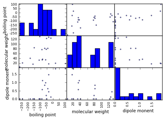
沸点、分子量、双極子モーメントがどのような関係にあるか散布図行列で概観してみましょう。
%matplotlib inline
import matplotlib.pyplot as plt
from pandas.tools.plotting import *
scatter_matrix(df)
plt.show()
まずは一番便利な scikit-learn から
前回、scikit-learnを使えば簡単に線形回帰できることをお示ししました。変数が増えて線形重回帰になっても、ほとんど手間が増えません。そう、scikit-learnならね。
from sklearn import linear_model
lr = linear_model.LinearRegression()
lr.fit(X, Y)
LinearRegression(copy_X=True, fit_intercept=True, n_jobs=1, normalize=False)
# 回帰係数
lr.coef_
array([ 1.17775083, 124.38195483])
# 切片
lr.intercept_
-218.85778226168119
print("y = f(x) = w1x1 + w2x2 + t; (w1, w2, t) = ({0}, {1}, {2})".format(lr.coef_[0], lr.coef_[1], lr.intercept_))
y = f(x) = w1x1 + w2x2 + t; (w1, w2, t) = (1.1777508314139944, 124.38195482549655, -218.8577822616812)
# 決定係数
lr.score(X, Y)
0.78084985722905187
lr.predict([200, 0.5])
array([ 78.88336143])
lr.predict([[150, 0], [100, 1.0]])
array([-42.19515755, 23.29925571])
次は、ガチPythonで。
scikit-learnを使わずにガチPythonで解こうと思うと、少し大変ですね。頑張ってみましょう。
# 平均値を求める関数
def mean(list):
    sum = 0
    for x in list:
        sum += x
    return sum / len(list)
# 分散を求める関数
def variance(list):
    ave = mean(list)
    sum = 0
    for x in list:
        sum += (x - ave) ** 2
    return sum / len(list)
# 標準偏差を求める関数
import math
def standard_deviation(list):
    return math.sqrt(variance(list))
# 共分散 = 偏差積の平均
def covariance(list1, list2):
    mean1 = mean(list1)
    mean2 = mean(list2)
    sum = 0
    for d1, d2 in zip(list1, list2):
        sum += (d1 - mean1) * (d2 - mean2)
    return sum / len(list1)
# 相関係数 = 共分散を list1, list2 の標準偏差で割ったもの
def correlation(list1, list2):
    return covariance(list1, list2) / (standard_deviation(list1) * standard_deviation(list2))
# a の影響を除いた、b と y の偏回帰係数 partial regression coefficient を求める関数
def partial_regression(a, b, y):
    rby = correlation(b, y)
    ray = correlation(a, y)
    rab = correlation(a, b)
    return (rby - ray * rab) * standard_deviation(y) / ((1 - rab ** 2) * standard_deviation(b))
# 定数 w1 = (x2 の影響を除いた、x1 と y の偏回帰係数)
w1 = partial_regression(X[:, 1], X[:, 0], Y)
# 定数 w2 = (x1 の影響を除いた、x2 と y の偏回帰係数)
w2 = partial_regression(X[:, 0], X[:, 1], Y)
# 定数 t = yの平均 - w1*x1の平均 - w2*x2の平均
t = mean(Y) - w1 * mean(X[:, 0]) - w2 * mean(X[:, 1])
# 回帰直線の式を表示
print("y = f(x) = w1x1 + w2x2 + t; (w1, w2, t) = ({0}, {1}, {2})".format(w1, w2, t))
y = f(x) = w1x1 + w2x2 + t; (w1, w2, t) = (1.1777508314139928, 124.38195482549644, -218.85778226168105)
def f(X):
    return w1 * X[:, 0] + w2 * X[:, 1] + t
r2 = 1. - sum((Y - f(X))**2) / sum((Y - mean(Y))**2)
r2
0.78084985722905187
さて、表計算で解けと言われたので pandas で書いてみましょうか。
二度とやりたくないくらい大変です。さあどうぞ。
import copy
from IPython.display import display
excel = copy.deepcopy(df)
excel
| molecule | boiling point | molecular weight | dipole monent | |
|---|---|---|---|---|
| 0 | HF | 19.500 | 20.0 | 1.826567 |
| 1 | HCl | -84.900 | 36.5 | 1.108600 |
| 2 | HBr | -67.000 | 80.9 | 0.827100 |
| 3 | HI | -35.100 | 127.9 | 0.447700 |
| 4 | H2O | 100.000 | 18.0 | 1.854600 |
| 5 | H2S | -60.700 | 34.1 | 0.978325 |
| 6 | H2Se | -42.000 | 81.0 | 0.627000 |
| 7 | NH3 | -33.400 | 17.0 | 1.471772 |
| 8 | PH3 | -87.000 | 34.0 | 0.573970 |
| 9 | AsH3 | -55.000 | 77.9 | 0.217000 |
| 10 | SbH3 | -17.100 | 124.8 | 0.116000 |
| 11 | CH4 | -161.490 | 16.0 | 0.000000 |
| 12 | SiH4 | -111.800 | 32.1 | 0.000000 |
| 13 | GeH4 | -90.000 | 76.6 | 0.000000 |
| 14 | SnH4 | -52.000 | 122.7 | 0.000000 |
| 15 | He | -268.934 | 4.0 | 0.000000 |
| 16 | Ne | -246.048 | 20.2 | 0.000000 |
| 17 | Ar | -185.700 | 39.9 | 0.000000 |
| 18 | Kr | -152.300 | 83.8 | 0.000000 |
| 19 | Xe | -108.100 | 131.3 | 0.000000 |
excel['y'] = excel['boiling point']
excel['x1'] = excel['molecular weight']
excel['x2'] = excel['dipole monent']
mean_y = mean(excel['y'])
mean_x1 = mean(excel['x1'])
mean_x2 = mean(excel['x2'])
display(excel, pd.DataFrame([[mean_y, mean_x1, mean_x2]], columns=['y','x1', 'x2'], index=['mean']))
| molecule | boiling point | molecular weight | dipole monent | y | x1 | x2 | |
|---|---|---|---|---|---|---|---|
| 0 | HF | 19.500 | 20.0 | 1.826567 | 19.500 | 20.0 | 1.826567 |
| 1 | HCl | -84.900 | 36.5 | 1.108600 | -84.900 | 36.5 | 1.108600 |
| 2 | HBr | -67.000 | 80.9 | 0.827100 | -67.000 | 80.9 | 0.827100 |
| 3 | HI | -35.100 | 127.9 | 0.447700 | -35.100 | 127.9 | 0.447700 |
| 4 | H2O | 100.000 | 18.0 | 1.854600 | 100.000 | 18.0 | 1.854600 |
| 5 | H2S | -60.700 | 34.1 | 0.978325 | -60.700 | 34.1 | 0.978325 |
| 6 | H2Se | -42.000 | 81.0 | 0.627000 | -42.000 | 81.0 | 0.627000 |
| 7 | NH3 | -33.400 | 17.0 | 1.471772 | -33.400 | 17.0 | 1.471772 |
| 8 | PH3 | -87.000 | 34.0 | 0.573970 | -87.000 | 34.0 | 0.573970 |
| 9 | AsH3 | -55.000 | 77.9 | 0.217000 | -55.000 | 77.9 | 0.217000 |
| 10 | SbH3 | -17.100 | 124.8 | 0.116000 | -17.100 | 124.8 | 0.116000 |
| 11 | CH4 | -161.490 | 16.0 | 0.000000 | -161.490 | 16.0 | 0.000000 |
| 12 | SiH4 | -111.800 | 32.1 | 0.000000 | -111.800 | 32.1 | 0.000000 |
| 13 | GeH4 | -90.000 | 76.6 | 0.000000 | -90.000 | 76.6 | 0.000000 |
| 14 | SnH4 | -52.000 | 122.7 | 0.000000 | -52.000 | 122.7 | 0.000000 |
| 15 | He | -268.934 | 4.0 | 0.000000 | -268.934 | 4.0 | 0.000000 |
| 16 | Ne | -246.048 | 20.2 | 0.000000 | -246.048 | 20.2 | 0.000000 |
| 17 | Ar | -185.700 | 39.9 | 0.000000 | -185.700 | 39.9 | 0.000000 |
| 18 | Kr | -152.300 | 83.8 | 0.000000 | -152.300 | 83.8 | 0.000000 |
| 19 | Xe | -108.100 | 131.3 | 0.000000 | -108.100 | 131.3 | 0.000000 |
| y | x1 | x2 | |
|---|---|---|---|
| mean | -86.9536 | 58.935 | 0.502432 |
excel['y-mean(y)'] = [y - mean_y for y in excel['y']]
excel['x1-mean(x1)'] = [x1 - mean_x1 for x1 in excel['x1']]
excel['x2-mean(x2)'] = [x2 - mean_x2 for x2 in excel['x2']]
display(excel, pd.DataFrame([[mean_y, mean_x1, mean_x2]], columns=['y','x1', 'x2'], index=['mean']))
| molecule | boiling point | molecular weight | dipole monent | y | x1 | x2 | y-mean(y) | x1-mean(x1) | x2-mean(x2) | |
|---|---|---|---|---|---|---|---|---|---|---|
| 0 | HF | 19.500 | 20.0 | 1.826567 | 19.500 | 20.0 | 1.826567 | 106.4536 | -38.935 | 1.324135 |
| 1 | HCl | -84.900 | 36.5 | 1.108600 | -84.900 | 36.5 | 1.108600 | 2.0536 | -22.435 | 0.606168 |
| 2 | HBr | -67.000 | 80.9 | 0.827100 | -67.000 | 80.9 | 0.827100 | 19.9536 | 21.965 | 0.324668 |
| 3 | HI | -35.100 | 127.9 | 0.447700 | -35.100 | 127.9 | 0.447700 | 51.8536 | 68.965 | -0.054732 |
| 4 | H2O | 100.000 | 18.0 | 1.854600 | 100.000 | 18.0 | 1.854600 | 186.9536 | -40.935 | 1.352168 |
| 5 | H2S | -60.700 | 34.1 | 0.978325 | -60.700 | 34.1 | 0.978325 | 26.2536 | -24.835 | 0.475893 |
| 6 | H2Se | -42.000 | 81.0 | 0.627000 | -42.000 | 81.0 | 0.627000 | 44.9536 | 22.065 | 0.124568 |
| 7 | NH3 | -33.400 | 17.0 | 1.471772 | -33.400 | 17.0 | 1.471772 | 53.5536 | -41.935 | 0.969340 |
| 8 | PH3 | -87.000 | 34.0 | 0.573970 | -87.000 | 34.0 | 0.573970 | -0.0464 | -24.935 | 0.071538 |
| 9 | AsH3 | -55.000 | 77.9 | 0.217000 | -55.000 | 77.9 | 0.217000 | 31.9536 | 18.965 | -0.285432 |
| 10 | SbH3 | -17.100 | 124.8 | 0.116000 | -17.100 | 124.8 | 0.116000 | 69.8536 | 65.865 | -0.386432 |
| 11 | CH4 | -161.490 | 16.0 | 0.000000 | -161.490 | 16.0 | 0.000000 | -74.5364 | -42.935 | -0.502432 |
| 12 | SiH4 | -111.800 | 32.1 | 0.000000 | -111.800 | 32.1 | 0.000000 | -24.8464 | -26.835 | -0.502432 |
| 13 | GeH4 | -90.000 | 76.6 | 0.000000 | -90.000 | 76.6 | 0.000000 | -3.0464 | 17.665 | -0.502432 |
| 14 | SnH4 | -52.000 | 122.7 | 0.000000 | -52.000 | 122.7 | 0.000000 | 34.9536 | 63.765 | -0.502432 |
| 15 | He | -268.934 | 4.0 | 0.000000 | -268.934 | 4.0 | 0.000000 | -181.9804 | -54.935 | -0.502432 |
| 16 | Ne | -246.048 | 20.2 | 0.000000 | -246.048 | 20.2 | 0.000000 | -159.0944 | -38.735 | -0.502432 |
| 17 | Ar | -185.700 | 39.9 | 0.000000 | -185.700 | 39.9 | 0.000000 | -98.7464 | -19.035 | -0.502432 |
| 18 | Kr | -152.300 | 83.8 | 0.000000 | -152.300 | 83.8 | 0.000000 | -65.3464 | 24.865 | -0.502432 |
| 19 | Xe | -108.100 | 131.3 | 0.000000 | -108.100 | 131.3 | 0.000000 | -21.1464 | 72.365 | -0.502432 |
| y | x1 | x2 | |
|---|---|---|---|
| mean | -86.9536 | 58.935 | 0.502432 |
excel['(y-mean(y))**2'] = [sa ** 2 for sa in excel['y-mean(y)']]
excel['(x1-mean(x1))**2'] = [sa ** 2 for sa in excel['x1-mean(x1)']]
excel['(x2-mean(x2))**2'] = [sa ** 2 for sa in excel['x2-mean(x2)']]
display(excel, pd.DataFrame([[mean_y, mean_x1, mean_x2]], columns=['y','x1', 'x2'], index=['mean']))
| molecule | boiling point | molecular weight | dipole monent | y | x1 | x2 | y-mean(y) | x1-mean(x1) | x2-mean(x2) | (y-mean(y))**2 | (x1-mean(x1))**2 | (x2-mean(x2))**2 | |
|---|---|---|---|---|---|---|---|---|---|---|---|---|---|
| 0 | HF | 19.500 | 20.0 | 1.826567 | 19.500 | 20.0 | 1.826567 | 106.4536 | -38.935 | 1.324135 | 11332.368953 | 1515.934225 | 1.753334 |
| 1 | HCl | -84.900 | 36.5 | 1.108600 | -84.900 | 36.5 | 1.108600 | 2.0536 | -22.435 | 0.606168 | 4.217273 | 503.329225 | 0.367440 |
| 2 | HBr | -67.000 | 80.9 | 0.827100 | -67.000 | 80.9 | 0.827100 | 19.9536 | 21.965 | 0.324668 | 398.146153 | 482.461225 | 0.105410 |
| 3 | HI | -35.100 | 127.9 | 0.447700 | -35.100 | 127.9 | 0.447700 | 51.8536 | 68.965 | -0.054732 | 2688.795833 | 4756.171225 | 0.002996 |
| 4 | H2O | 100.000 | 18.0 | 1.854600 | 100.000 | 18.0 | 1.854600 | 186.9536 | -40.935 | 1.352168 | 34951.648553 | 1675.674225 | 1.828359 |
| 5 | H2S | -60.700 | 34.1 | 0.978325 | -60.700 | 34.1 | 0.978325 | 26.2536 | -24.835 | 0.475893 | 689.251513 | 616.777225 | 0.226474 |
| 6 | H2Se | -42.000 | 81.0 | 0.627000 | -42.000 | 81.0 | 0.627000 | 44.9536 | 22.065 | 0.124568 | 2020.826153 | 486.864225 | 0.015517 |
| 7 | NH3 | -33.400 | 17.0 | 1.471772 | -33.400 | 17.0 | 1.471772 | 53.5536 | -41.935 | 0.969340 | 2867.988073 | 1758.544225 | 0.939621 |
| 8 | PH3 | -87.000 | 34.0 | 0.573970 | -87.000 | 34.0 | 0.573970 | -0.0464 | -24.935 | 0.071538 | 0.002153 | 621.754225 | 0.005118 |
| 9 | AsH3 | -55.000 | 77.9 | 0.217000 | -55.000 | 77.9 | 0.217000 | 31.9536 | 18.965 | -0.285432 | 1021.032553 | 359.671225 | 0.081471 |
| 10 | SbH3 | -17.100 | 124.8 | 0.116000 | -17.100 | 124.8 | 0.116000 | 69.8536 | 65.865 | -0.386432 | 4879.525433 | 4338.198225 | 0.149329 |
| 11 | CH4 | -161.490 | 16.0 | 0.000000 | -161.490 | 16.0 | 0.000000 | -74.5364 | -42.935 | -0.502432 | 5555.674925 | 1843.414225 | 0.252438 |
| 12 | SiH4 | -111.800 | 32.1 | 0.000000 | -111.800 | 32.1 | 0.000000 | -24.8464 | -26.835 | -0.502432 | 617.343593 | 720.117225 | 0.252438 |
| 13 | GeH4 | -90.000 | 76.6 | 0.000000 | -90.000 | 76.6 | 0.000000 | -3.0464 | 17.665 | -0.502432 | 9.280553 | 312.052225 | 0.252438 |
| 14 | SnH4 | -52.000 | 122.7 | 0.000000 | -52.000 | 122.7 | 0.000000 | 34.9536 | 63.765 | -0.502432 | 1221.754153 | 4065.975225 | 0.252438 |
| 15 | He | -268.934 | 4.0 | 0.000000 | -268.934 | 4.0 | 0.000000 | -181.9804 | -54.935 | -0.502432 | 33116.865984 | 3017.854225 | 0.252438 |
| 16 | Ne | -246.048 | 20.2 | 0.000000 | -246.048 | 20.2 | 0.000000 | -159.0944 | -38.735 | -0.502432 | 25311.028111 | 1500.400225 | 0.252438 |
| 17 | Ar | -185.700 | 39.9 | 0.000000 | -185.700 | 39.9 | 0.000000 | -98.7464 | -19.035 | -0.502432 | 9750.851513 | 362.331225 | 0.252438 |
| 18 | Kr | -152.300 | 83.8 | 0.000000 | -152.300 | 83.8 | 0.000000 | -65.3464 | 24.865 | -0.502432 | 4270.151993 | 618.268225 | 0.252438 |
| 19 | Xe | -108.100 | 131.3 | 0.000000 | -108.100 | 131.3 | 0.000000 | -21.1464 | 72.365 | -0.502432 | 447.170233 | 5236.693225 | 0.252438 |
| y | x1 | x2 | |
|---|---|---|---|
| mean | -86.9536 | 58.935 | 0.502432 |
variance_y = mean(excel['(y-mean(y))**2'])
variance_x1 = mean(excel['(x1-mean(x1))**2'])
variance_x2 = mean(excel['(x2-mean(x2))**2'])
sd_y = math.sqrt(variance_y)
sd_x1 = math.sqrt(variance_x1)
sd_x2 = math.sqrt(variance_x2)
display(excel, pd.DataFrame([[mean_y, mean_x1, mean_x2],
                             [variance_y, variance_x1, variance_x2],
                             [sd_y, sd_x1, sd_x2]],
                            columns=['y','x1', 'x2'], index=['mean', 'variance', 'sd']))
| molecule | boiling point | molecular weight | dipole monent | y | x1 | x2 | y-mean(y) | x1-mean(x1) | x2-mean(x2) | (y-mean(y))**2 | (x1-mean(x1))**2 | (x2-mean(x2))**2 | |
|---|---|---|---|---|---|---|---|---|---|---|---|---|---|
| 0 | HF | 19.500 | 20.0 | 1.826567 | 19.500 | 20.0 | 1.826567 | 106.4536 | -38.935 | 1.324135 | 11332.368953 | 1515.934225 | 1.753334 |
| 1 | HCl | -84.900 | 36.5 | 1.108600 | -84.900 | 36.5 | 1.108600 | 2.0536 | -22.435 | 0.606168 | 4.217273 | 503.329225 | 0.367440 |
| 2 | HBr | -67.000 | 80.9 | 0.827100 | -67.000 | 80.9 | 0.827100 | 19.9536 | 21.965 | 0.324668 | 398.146153 | 482.461225 | 0.105410 |
| 3 | HI | -35.100 | 127.9 | 0.447700 | -35.100 | 127.9 | 0.447700 | 51.8536 | 68.965 | -0.054732 | 2688.795833 | 4756.171225 | 0.002996 |
| 4 | H2O | 100.000 | 18.0 | 1.854600 | 100.000 | 18.0 | 1.854600 | 186.9536 | -40.935 | 1.352168 | 34951.648553 | 1675.674225 | 1.828359 |
| 5 | H2S | -60.700 | 34.1 | 0.978325 | -60.700 | 34.1 | 0.978325 | 26.2536 | -24.835 | 0.475893 | 689.251513 | 616.777225 | 0.226474 |
| 6 | H2Se | -42.000 | 81.0 | 0.627000 | -42.000 | 81.0 | 0.627000 | 44.9536 | 22.065 | 0.124568 | 2020.826153 | 486.864225 | 0.015517 |
| 7 | NH3 | -33.400 | 17.0 | 1.471772 | -33.400 | 17.0 | 1.471772 | 53.5536 | -41.935 | 0.969340 | 2867.988073 | 1758.544225 | 0.939621 |
| 8 | PH3 | -87.000 | 34.0 | 0.573970 | -87.000 | 34.0 | 0.573970 | -0.0464 | -24.935 | 0.071538 | 0.002153 | 621.754225 | 0.005118 |
| 9 | AsH3 | -55.000 | 77.9 | 0.217000 | -55.000 | 77.9 | 0.217000 | 31.9536 | 18.965 | -0.285432 | 1021.032553 | 359.671225 | 0.081471 |
| 10 | SbH3 | -17.100 | 124.8 | 0.116000 | -17.100 | 124.8 | 0.116000 | 69.8536 | 65.865 | -0.386432 | 4879.525433 | 4338.198225 | 0.149329 |
| 11 | CH4 | -161.490 | 16.0 | 0.000000 | -161.490 | 16.0 | 0.000000 | -74.5364 | -42.935 | -0.502432 | 5555.674925 | 1843.414225 | 0.252438 |
| 12 | SiH4 | -111.800 | 32.1 | 0.000000 | -111.800 | 32.1 | 0.000000 | -24.8464 | -26.835 | -0.502432 | 617.343593 | 720.117225 | 0.252438 |
| 13 | GeH4 | -90.000 | 76.6 | 0.000000 | -90.000 | 76.6 | 0.000000 | -3.0464 | 17.665 | -0.502432 | 9.280553 | 312.052225 | 0.252438 |
| 14 | SnH4 | -52.000 | 122.7 | 0.000000 | -52.000 | 122.7 | 0.000000 | 34.9536 | 63.765 | -0.502432 | 1221.754153 | 4065.975225 | 0.252438 |
| 15 | He | -268.934 | 4.0 | 0.000000 | -268.934 | 4.0 | 0.000000 | -181.9804 | -54.935 | -0.502432 | 33116.865984 | 3017.854225 | 0.252438 |
| 16 | Ne | -246.048 | 20.2 | 0.000000 | -246.048 | 20.2 | 0.000000 | -159.0944 | -38.735 | -0.502432 | 25311.028111 | 1500.400225 | 0.252438 |
| 17 | Ar | -185.700 | 39.9 | 0.000000 | -185.700 | 39.9 | 0.000000 | -98.7464 | -19.035 | -0.502432 | 9750.851513 | 362.331225 | 0.252438 |
| 18 | Kr | -152.300 | 83.8 | 0.000000 | -152.300 | 83.8 | 0.000000 | -65.3464 | 24.865 | -0.502432 | 4270.151993 | 618.268225 | 0.252438 |
| 19 | Xe | -108.100 | 131.3 | 0.000000 | -108.100 | 131.3 | 0.000000 | -21.1464 | 72.365 | -0.502432 | 447.170233 | 5236.693225 | 0.252438 |
| y | x1 | x2 | |
|---|---|---|---|
| mean | -86.953600 | 58.935000 | 0.502432 |
| variance | 7057.696185 | 1739.624275 | 0.387350 |
| sd | 84.010096 | 41.708803 | 0.622375 |
excel['(x1-mean(x1)) * (x2-mean(x2))'] = excel['x1-mean(x1)'] * excel['x2-mean(x2)']
excel['(y-mean(y)) * (x1-mean(x1))'] = excel['y-mean(y)'] * excel['x1-mean(x1)']
excel['(y-mean(y)) * (x2-mean(x2))'] = excel['y-mean(y)'] * excel['x2-mean(x2)']
display(excel, pd.DataFrame([[mean_y, mean_x1, mean_x2],
                             [variance_y, variance_x1, variance_x2],
                             [sd_y, sd_x1, sd_x2]],
                            columns=['y','x1', 'x2'], index=['mean', 'variance', 'sd']))
| molecule | boiling point | molecular weight | dipole monent | y | x1 | x2 | y-mean(y) | x1-mean(x1) | x2-mean(x2) | (y-mean(y))**2 | (x1-mean(x1))**2 | (x2-mean(x2))**2 | (x1-mean(x1)) * (x2-mean(x2)) | (y-mean(y)) * (x1-mean(x1)) | (y-mean(y)) * (x2-mean(x2)) | |
|---|---|---|---|---|---|---|---|---|---|---|---|---|---|---|---|---|
| 0 | HF | 19.500 | 20.0 | 1.826567 | 19.500 | 20.0 | 1.826567 | 106.4536 | -38.935 | 1.324135 | 11332.368953 | 1515.934225 | 1.753334 | -51.555208 | -4144.770916 | 140.958970 |
| 1 | HCl | -84.900 | 36.5 | 1.108600 | -84.900 | 36.5 | 1.108600 | 2.0536 | -22.435 | 0.606168 | 4.217273 | 503.329225 | 0.367440 | -13.599386 | -46.072516 | 1.244827 |
| 2 | HBr | -67.000 | 80.9 | 0.827100 | -67.000 | 80.9 | 0.827100 | 19.9536 | 21.965 | 0.324668 | 398.146153 | 482.461225 | 0.105410 | 7.131339 | 438.280824 | 6.478301 |
| 3 | HI | -35.100 | 127.9 | 0.447700 | -35.100 | 127.9 | 0.447700 | 51.8536 | 68.965 | -0.054732 | 2688.795833 | 4756.171225 | 0.002996 | -3.774572 | 3576.083524 | -2.838036 |
| 4 | H2O | 100.000 | 18.0 | 1.854600 | 100.000 | 18.0 | 1.854600 | 186.9536 | -40.935 | 1.352168 | 34951.648553 | 1675.674225 | 1.828359 | -55.351009 | -7652.945616 | 252.792731 |
| 5 | H2S | -60.700 | 34.1 | 0.978325 | -60.700 | 34.1 | 0.978325 | 26.2536 | -24.835 | 0.475893 | 689.251513 | 616.777225 | 0.226474 | -11.818810 | -652.008156 | 12.493912 |
| 6 | H2Se | -42.000 | 81.0 | 0.627000 | -42.000 | 81.0 | 0.627000 | 44.9536 | 22.065 | 0.124568 | 2020.826153 | 486.864225 | 0.015517 | 2.748600 | 991.901184 | 5.599794 |
| 7 | NH3 | -33.400 | 17.0 | 1.471772 | -33.400 | 17.0 | 1.471772 | 53.5536 | -41.935 | 0.969340 | 2867.988073 | 1758.544225 | 0.939621 | -40.649285 | -2245.770216 | 51.911663 |
| 8 | PH3 | -87.000 | 34.0 | 0.573970 | -87.000 | 34.0 | 0.573970 | -0.0464 | -24.935 | 0.071538 | 0.002153 | 621.754225 | 0.005118 | -1.783808 | 1.156984 | -0.003319 |
| 9 | AsH3 | -55.000 | 77.9 | 0.217000 | -55.000 | 77.9 | 0.217000 | 31.9536 | 18.965 | -0.285432 | 1021.032553 | 359.671225 | 0.081471 | -5.413212 | 606.000024 | -9.120570 |
| 10 | SbH3 | -17.100 | 124.8 | 0.116000 | -17.100 | 124.8 | 0.116000 | 69.8536 | 65.865 | -0.386432 | 4879.525433 | 4338.198225 | 0.149329 | -25.452324 | 4600.907364 | -26.993645 |
| 11 | CH4 | -161.490 | 16.0 | 0.000000 | -161.490 | 16.0 | 0.000000 | -74.5364 | -42.935 | -0.502432 | 5555.674925 | 1843.414225 | 0.252438 | 21.571905 | 3200.220334 | 37.449450 |
| 12 | SiH4 | -111.800 | 32.1 | 0.000000 | -111.800 | 32.1 | 0.000000 | -24.8464 | -26.835 | -0.502432 | 617.343593 | 720.117225 | 0.252438 | 13.482755 | 666.753144 | 12.483619 |
| 13 | GeH4 | -90.000 | 76.6 | 0.000000 | -90.000 | 76.6 | 0.000000 | -3.0464 | 17.665 | -0.502432 | 9.280553 | 312.052225 | 0.252438 | -8.875456 | -53.814656 | 1.530608 |
| 14 | SnH4 | -52.000 | 122.7 | 0.000000 | -52.000 | 122.7 | 0.000000 | 34.9536 | 63.765 | -0.502432 | 1221.754153 | 4065.975225 | 0.252438 | -32.037557 | 2228.816304 | -17.561797 |
| 15 | He | -268.934 | 4.0 | 0.000000 | -268.934 | 4.0 | 0.000000 | -181.9804 | -54.935 | -0.502432 | 33116.865984 | 3017.854225 | 0.252438 | 27.601085 | 9997.093274 | 91.432722 |
| 16 | Ne | -246.048 | 20.2 | 0.000000 | -246.048 | 20.2 | 0.000000 | -159.0944 | -38.735 | -0.502432 | 25311.028111 | 1500.400225 | 0.252438 | 19.461692 | 6162.521584 | 79.934070 |
| 17 | Ar | -185.700 | 39.9 | 0.000000 | -185.700 | 39.9 | 0.000000 | -98.7464 | -19.035 | -0.502432 | 9750.851513 | 362.331225 | 0.252438 | 9.563787 | 1879.637724 | 49.613322 |
| 18 | Kr | -152.300 | 83.8 | 0.000000 | -152.300 | 83.8 | 0.000000 | -65.3464 | 24.865 | -0.502432 | 4270.151993 | 618.268225 | 0.252438 | -12.492964 | -1624.838236 | 32.832103 |
| 19 | Xe | -108.100 | 131.3 | 0.000000 | -108.100 | 131.3 | 0.000000 | -21.1464 | 72.365 | -0.502432 | 447.170233 | 5236.693225 | 0.252438 | -36.358470 | -1530.259236 | 10.624622 |
| y | x1 | x2 | |
|---|---|---|---|
| mean | -86.953600 | 58.935000 | 0.502432 |
| variance | 7057.696185 | 1739.624275 | 0.387350 |
| sd | 84.010096 | 41.708803 | 0.622375 |
covar_x1x2 = mean(excel['(x1-mean(x1)) * (x2-mean(x2))'])
covar_x1y = mean(excel['(y-mean(y)) * (x1-mean(x1))'])
covar_x2y = mean(excel['(y-mean(y)) * (x2-mean(x2))'])

corr_x1x2 = covar_x1x2 / (sd_x1 * sd_x2)
corr_x1y = covar_x1y / (sd_x1 * sd_y)
corr_x2y = covar_x2y / (sd_x2 * sd_y)
display(excel, pd.DataFrame([[mean_y, mean_x1, mean_x2],
                             [variance_y, variance_x1, variance_x2],
                             [sd_y, sd_x1, sd_x2]],
                            columns=['y','x1', 'x2'], index=['mean', 'variance', 'sd']),
       pd.DataFrame([[covar_x1x2, covar_x1y, covar_x2y], [corr_x1x2, corr_x1y, corr_x2y]],
                    index=['covariance', 'correlation'], columns=['x1,x2','x1,y', 'x2,y']))
| molecule | boiling point | molecular weight | dipole monent | y | x1 | x2 | y-mean(y) | x1-mean(x1) | x2-mean(x2) | (y-mean(y))**2 | (x1-mean(x1))**2 | (x2-mean(x2))**2 | (x1-mean(x1)) * (x2-mean(x2)) | (y-mean(y)) * (x1-mean(x1)) | (y-mean(y)) * (x2-mean(x2)) | |
|---|---|---|---|---|---|---|---|---|---|---|---|---|---|---|---|---|
| 0 | HF | 19.500 | 20.0 | 1.826567 | 19.500 | 20.0 | 1.826567 | 106.4536 | -38.935 | 1.324135 | 11332.368953 | 1515.934225 | 1.753334 | -51.555208 | -4144.770916 | 140.958970 |
| 1 | HCl | -84.900 | 36.5 | 1.108600 | -84.900 | 36.5 | 1.108600 | 2.0536 | -22.435 | 0.606168 | 4.217273 | 503.329225 | 0.367440 | -13.599386 | -46.072516 | 1.244827 |
| 2 | HBr | -67.000 | 80.9 | 0.827100 | -67.000 | 80.9 | 0.827100 | 19.9536 | 21.965 | 0.324668 | 398.146153 | 482.461225 | 0.105410 | 7.131339 | 438.280824 | 6.478301 |
| 3 | HI | -35.100 | 127.9 | 0.447700 | -35.100 | 127.9 | 0.447700 | 51.8536 | 68.965 | -0.054732 | 2688.795833 | 4756.171225 | 0.002996 | -3.774572 | 3576.083524 | -2.838036 |
| 4 | H2O | 100.000 | 18.0 | 1.854600 | 100.000 | 18.0 | 1.854600 | 186.9536 | -40.935 | 1.352168 | 34951.648553 | 1675.674225 | 1.828359 | -55.351009 | -7652.945616 | 252.792731 |
| 5 | H2S | -60.700 | 34.1 | 0.978325 | -60.700 | 34.1 | 0.978325 | 26.2536 | -24.835 | 0.475893 | 689.251513 | 616.777225 | 0.226474 | -11.818810 | -652.008156 | 12.493912 |
| 6 | H2Se | -42.000 | 81.0 | 0.627000 | -42.000 | 81.0 | 0.627000 | 44.9536 | 22.065 | 0.124568 | 2020.826153 | 486.864225 | 0.015517 | 2.748600 | 991.901184 | 5.599794 |
| 7 | NH3 | -33.400 | 17.0 | 1.471772 | -33.400 | 17.0 | 1.471772 | 53.5536 | -41.935 | 0.969340 | 2867.988073 | 1758.544225 | 0.939621 | -40.649285 | -2245.770216 | 51.911663 |
| 8 | PH3 | -87.000 | 34.0 | 0.573970 | -87.000 | 34.0 | 0.573970 | -0.0464 | -24.935 | 0.071538 | 0.002153 | 621.754225 | 0.005118 | -1.783808 | 1.156984 | -0.003319 |
| 9 | AsH3 | -55.000 | 77.9 | 0.217000 | -55.000 | 77.9 | 0.217000 | 31.9536 | 18.965 | -0.285432 | 1021.032553 | 359.671225 | 0.081471 | -5.413212 | 606.000024 | -9.120570 |
| 10 | SbH3 | -17.100 | 124.8 | 0.116000 | -17.100 | 124.8 | 0.116000 | 69.8536 | 65.865 | -0.386432 | 4879.525433 | 4338.198225 | 0.149329 | -25.452324 | 4600.907364 | -26.993645 |
| 11 | CH4 | -161.490 | 16.0 | 0.000000 | -161.490 | 16.0 | 0.000000 | -74.5364 | -42.935 | -0.502432 | 5555.674925 | 1843.414225 | 0.252438 | 21.571905 | 3200.220334 | 37.449450 |
| 12 | SiH4 | -111.800 | 32.1 | 0.000000 | -111.800 | 32.1 | 0.000000 | -24.8464 | -26.835 | -0.502432 | 617.343593 | 720.117225 | 0.252438 | 13.482755 | 666.753144 | 12.483619 |
| 13 | GeH4 | -90.000 | 76.6 | 0.000000 | -90.000 | 76.6 | 0.000000 | -3.0464 | 17.665 | -0.502432 | 9.280553 | 312.052225 | 0.252438 | -8.875456 | -53.814656 | 1.530608 |
| 14 | SnH4 | -52.000 | 122.7 | 0.000000 | -52.000 | 122.7 | 0.000000 | 34.9536 | 63.765 | -0.502432 | 1221.754153 | 4065.975225 | 0.252438 | -32.037557 | 2228.816304 | -17.561797 |
| 15 | He | -268.934 | 4.0 | 0.000000 | -268.934 | 4.0 | 0.000000 | -181.9804 | -54.935 | -0.502432 | 33116.865984 | 3017.854225 | 0.252438 | 27.601085 | 9997.093274 | 91.432722 |
| 16 | Ne | -246.048 | 20.2 | 0.000000 | -246.048 | 20.2 | 0.000000 | -159.0944 | -38.735 | -0.502432 | 25311.028111 | 1500.400225 | 0.252438 | 19.461692 | 6162.521584 | 79.934070 |
| 17 | Ar | -185.700 | 39.9 | 0.000000 | -185.700 | 39.9 | 0.000000 | -98.7464 | -19.035 | -0.502432 | 9750.851513 | 362.331225 | 0.252438 | 9.563787 | 1879.637724 | 49.613322 |
| 18 | Kr | -152.300 | 83.8 | 0.000000 | -152.300 | 83.8 | 0.000000 | -65.3464 | 24.865 | -0.502432 | 4270.151993 | 618.268225 | 0.252438 | -12.492964 | -1624.838236 | 32.832103 |
| 19 | Xe | -108.100 | 131.3 | 0.000000 | -108.100 | 131.3 | 0.000000 | -21.1464 | 72.365 | -0.502432 | 447.170233 | 5236.693225 | 0.252438 | -36.358470 | -1530.259236 | 10.624622 |
| y | x1 | x2 | |
|---|---|---|---|
| mean | -86.953600 | 58.935000 | 0.502432 |
| variance | 7057.696185 | 1739.624275 | 0.387350 |
| sd | 84.010096 | 41.708803 | 0.622375 |
| x1,x2 | x1,y | x2,y | |
|---|---|---|---|
| covariance | -9.880045 | 819.944636 | 36.543167 |
| correlation | -0.380609 | 0.234005 | 0.698912 |
w1 = (corr_x1y - corr_x2y * corr_x1x2) * sd_y / ((1 - corr_x1x2 ** 2) * sd_x1)
w2 = (corr_x2y - corr_x1y * corr_x1x2) * sd_y / ((1 - corr_x1x2 ** 2) * sd_x2)
t = mean_y - w1 * mean_x1 - w2 * mean_x2
display(excel,
        pd.DataFrame([[mean_y, mean_x1, mean_x2],
                      [variance_y, variance_x1, variance_x2],
                      [sd_y, sd_x1, sd_x2]],
                     columns=['y','x1', 'x2'], index=['mean', 'variance', 'sd']),
        pd.DataFrame([[covar_x1x2, covar_x1y, covar_x2y], [corr_x1x2, corr_x1y, corr_x2y]],
                     index=['covariance', 'correlation'], columns=['x1,x2','x1,y', 'x2,y']),
        pd.DataFrame([[w1, w2, t]], columns=["w1", "w2", "t"], index=["y = f(x) = w1x1 + w2x2 + t"]))
| molecule | boiling point | molecular weight | dipole monent | y | x1 | x2 | y-mean(y) | x1-mean(x1) | x2-mean(x2) | (y-mean(y))**2 | (x1-mean(x1))**2 | (x2-mean(x2))**2 | (x1-mean(x1)) * (x2-mean(x2)) | (y-mean(y)) * (x1-mean(x1)) | (y-mean(y)) * (x2-mean(x2)) | |
|---|---|---|---|---|---|---|---|---|---|---|---|---|---|---|---|---|
| 0 | HF | 19.500 | 20.0 | 1.826567 | 19.500 | 20.0 | 1.826567 | 106.4536 | -38.935 | 1.324135 | 11332.368953 | 1515.934225 | 1.753334 | -51.555208 | -4144.770916 | 140.958970 |
| 1 | HCl | -84.900 | 36.5 | 1.108600 | -84.900 | 36.5 | 1.108600 | 2.0536 | -22.435 | 0.606168 | 4.217273 | 503.329225 | 0.367440 | -13.599386 | -46.072516 | 1.244827 |
| 2 | HBr | -67.000 | 80.9 | 0.827100 | -67.000 | 80.9 | 0.827100 | 19.9536 | 21.965 | 0.324668 | 398.146153 | 482.461225 | 0.105410 | 7.131339 | 438.280824 | 6.478301 |
| 3 | HI | -35.100 | 127.9 | 0.447700 | -35.100 | 127.9 | 0.447700 | 51.8536 | 68.965 | -0.054732 | 2688.795833 | 4756.171225 | 0.002996 | -3.774572 | 3576.083524 | -2.838036 |
| 4 | H2O | 100.000 | 18.0 | 1.854600 | 100.000 | 18.0 | 1.854600 | 186.9536 | -40.935 | 1.352168 | 34951.648553 | 1675.674225 | 1.828359 | -55.351009 | -7652.945616 | 252.792731 |
| 5 | H2S | -60.700 | 34.1 | 0.978325 | -60.700 | 34.1 | 0.978325 | 26.2536 | -24.835 | 0.475893 | 689.251513 | 616.777225 | 0.226474 | -11.818810 | -652.008156 | 12.493912 |
| 6 | H2Se | -42.000 | 81.0 | 0.627000 | -42.000 | 81.0 | 0.627000 | 44.9536 | 22.065 | 0.124568 | 2020.826153 | 486.864225 | 0.015517 | 2.748600 | 991.901184 | 5.599794 |
| 7 | NH3 | -33.400 | 17.0 | 1.471772 | -33.400 | 17.0 | 1.471772 | 53.5536 | -41.935 | 0.969340 | 2867.988073 | 1758.544225 | 0.939621 | -40.649285 | -2245.770216 | 51.911663 |
| 8 | PH3 | -87.000 | 34.0 | 0.573970 | -87.000 | 34.0 | 0.573970 | -0.0464 | -24.935 | 0.071538 | 0.002153 | 621.754225 | 0.005118 | -1.783808 | 1.156984 | -0.003319 |
| 9 | AsH3 | -55.000 | 77.9 | 0.217000 | -55.000 | 77.9 | 0.217000 | 31.9536 | 18.965 | -0.285432 | 1021.032553 | 359.671225 | 0.081471 | -5.413212 | 606.000024 | -9.120570 |
| 10 | SbH3 | -17.100 | 124.8 | 0.116000 | -17.100 | 124.8 | 0.116000 | 69.8536 | 65.865 | -0.386432 | 4879.525433 | 4338.198225 | 0.149329 | -25.452324 | 4600.907364 | -26.993645 |
| 11 | CH4 | -161.490 | 16.0 | 0.000000 | -161.490 | 16.0 | 0.000000 | -74.5364 | -42.935 | -0.502432 | 5555.674925 | 1843.414225 | 0.252438 | 21.571905 | 3200.220334 | 37.449450 |
| 12 | SiH4 | -111.800 | 32.1 | 0.000000 | -111.800 | 32.1 | 0.000000 | -24.8464 | -26.835 | -0.502432 | 617.343593 | 720.117225 | 0.252438 | 13.482755 | 666.753144 | 12.483619 |
| 13 | GeH4 | -90.000 | 76.6 | 0.000000 | -90.000 | 76.6 | 0.000000 | -3.0464 | 17.665 | -0.502432 | 9.280553 | 312.052225 | 0.252438 | -8.875456 | -53.814656 | 1.530608 |
| 14 | SnH4 | -52.000 | 122.7 | 0.000000 | -52.000 | 122.7 | 0.000000 | 34.9536 | 63.765 | -0.502432 | 1221.754153 | 4065.975225 | 0.252438 | -32.037557 | 2228.816304 | -17.561797 |
| 15 | He | -268.934 | 4.0 | 0.000000 | -268.934 | 4.0 | 0.000000 | -181.9804 | -54.935 | -0.502432 | 33116.865984 | 3017.854225 | 0.252438 | 27.601085 | 9997.093274 | 91.432722 |
| 16 | Ne | -246.048 | 20.2 | 0.000000 | -246.048 | 20.2 | 0.000000 | -159.0944 | -38.735 | -0.502432 | 25311.028111 | 1500.400225 | 0.252438 | 19.461692 | 6162.521584 | 79.934070 |
| 17 | Ar | -185.700 | 39.9 | 0.000000 | -185.700 | 39.9 | 0.000000 | -98.7464 | -19.035 | -0.502432 | 9750.851513 | 362.331225 | 0.252438 | 9.563787 | 1879.637724 | 49.613322 |
| 18 | Kr | -152.300 | 83.8 | 0.000000 | -152.300 | 83.8 | 0.000000 | -65.3464 | 24.865 | -0.502432 | 4270.151993 | 618.268225 | 0.252438 | -12.492964 | -1624.838236 | 32.832103 |
| 19 | Xe | -108.100 | 131.3 | 0.000000 | -108.100 | 131.3 | 0.000000 | -21.1464 | 72.365 | -0.502432 | 447.170233 | 5236.693225 | 0.252438 | -36.358470 | -1530.259236 | 10.624622 |
| y | x1 | x2 | |
|---|---|---|---|
| mean | -86.953600 | 58.935000 | 0.502432 |
| variance | 7057.696185 | 1739.624275 | 0.387350 |
| sd | 84.010096 | 41.708803 | 0.622375 |
| x1,x2 | x1,y | x2,y | |
|---|---|---|---|
| covariance | -9.880045 | 819.944636 | 36.543167 |
| correlation | -0.380609 | 0.234005 | 0.698912 |
| w1 | w2 | t | |
|---|---|---|---|
| y = f(x) = w1x1 + w2x2 + t | 1.177751 | 124.381955 | -218.857782 |
def f(x1, x2):
    return w1 * x1 + w2 * x2 + t
excel['f(x1,x2)'] = f(excel['x1'], excel['x2'])
display(excel,
        pd.DataFrame([[mean_y, mean_x1, mean_x2],
                      [variance_y, variance_x1, variance_x2],
                      [sd_y, sd_x1, sd_x2]],
                     columns=['y','x1', 'x2'], index=['mean', 'variance', 'sd']),
        pd.DataFrame([[covar_x1x2, covar_x1y, covar_x2y], [corr_x1x2, corr_x1y, corr_x2y]],
                     index=['covariance', 'correlation'], columns=['x1,x2','x1,y', 'x2,y']),
        pd.DataFrame([[w1, w2, t]], columns=["w1", "w2", "t"], index=["y = f(x) = w1x1 + w2x2 + t"]))
| molecule | boiling point | molecular weight | dipole monent | y | x1 | x2 | y-mean(y) | x1-mean(x1) | x2-mean(x2) | (y-mean(y))**2 | (x1-mean(x1))**2 | (x2-mean(x2))**2 | (x1-mean(x1)) * (x2-mean(x2)) | (y-mean(y)) * (x1-mean(x1)) | (y-mean(y)) * (x2-mean(x2)) | f(x1,x2) | |
|---|---|---|---|---|---|---|---|---|---|---|---|---|---|---|---|---|---|
| 0 | HF | 19.500 | 20.0 | 1.826567 | 19.500 | 20.0 | 1.826567 | 106.4536 | -38.935 | 1.324135 | 11332.368953 | 1515.934225 | 1.753334 | -51.555208 | -4144.770916 | 140.958970 | 31.889208 |
| 1 | HCl | -84.900 | 36.5 | 1.108600 | -84.900 | 36.5 | 1.108600 | 2.0536 | -22.435 | 0.606168 | 4.217273 | 503.329225 | 0.367440 | -13.599386 | -46.072516 | 1.244827 | -37.980042 |
| 2 | HBr | -67.000 | 80.9 | 0.827100 | -67.000 | 80.9 | 0.827100 | 19.9536 | 21.965 | 0.324668 | 398.146153 | 482.461225 | 0.105410 | 7.131339 | 438.280824 | 6.478301 | -20.701425 |
| 3 | HI | -35.100 | 127.9 | 0.447700 | -35.100 | 127.9 | 0.447700 | 51.8536 | 68.965 | -0.054732 | 2688.795833 | 4756.171225 | 0.002996 | -3.774572 | 3576.083524 | -2.838036 | -12.537650 |
| 4 | H2O | 100.000 | 18.0 | 1.854600 | 100.000 | 18.0 | 1.854600 | 186.9536 | -40.935 | 1.352168 | 34951.648553 | 1675.674225 | 1.828359 | -55.351009 | -7652.945616 | 252.792731 | 33.020506 |
| 5 | H2S | -60.700 | 34.1 | 0.978325 | -60.700 | 34.1 | 0.978325 | 26.2536 | -24.835 | 0.475893 | 689.251513 | 616.777225 | 0.226474 | -11.818810 | -652.008156 | 12.493912 | -57.010503 |
| 6 | H2Se | -42.000 | 81.0 | 0.627000 | -42.000 | 81.0 | 0.627000 | 44.9536 | 22.065 | 0.124568 | 2020.826153 | 486.864225 | 0.015517 | 2.748600 | 991.901184 | 5.599794 | -45.472479 |
| 7 | NH3 | -33.400 | 17.0 | 1.471772 | -33.400 | 17.0 | 1.471772 | 53.5536 | -41.935 | 0.969340 | 2867.988073 | 1758.544225 | 0.939621 | -40.649285 | -2245.770216 | 51.911663 | -15.774140 |
| 8 | PH3 | -87.000 | 34.0 | 0.573970 | -87.000 | 34.0 | 0.573970 | -0.0464 | -24.935 | 0.071538 | 0.002153 | 621.754225 | 0.005118 | -1.783808 | 1.156984 | -0.003319 | -107.422743 |
| 9 | AsH3 | -55.000 | 77.9 | 0.217000 | -55.000 | 77.9 | 0.217000 | 31.9536 | 18.965 | -0.285432 | 1021.032553 | 359.671225 | 0.081471 | -5.413212 | 606.000024 | -9.120570 | -100.120108 |
| 10 | SbH3 | -17.100 | 124.8 | 0.116000 | -17.100 | 124.8 | 0.116000 | 69.8536 | 65.865 | -0.386432 | 4879.525433 | 4338.198225 | 0.149329 | -25.452324 | 4600.907364 | -26.993645 | -57.446172 |
| 11 | CH4 | -161.490 | 16.0 | 0.000000 | -161.490 | 16.0 | 0.000000 | -74.5364 | -42.935 | -0.502432 | 5555.674925 | 1843.414225 | 0.252438 | 21.571905 | 3200.220334 | 37.449450 | -200.013769 |
| 12 | SiH4 | -111.800 | 32.1 | 0.000000 | -111.800 | 32.1 | 0.000000 | -24.8464 | -26.835 | -0.502432 | 617.343593 | 720.117225 | 0.252438 | 13.482755 | 666.753144 | 12.483619 | -181.051981 |
| 13 | GeH4 | -90.000 | 76.6 | 0.000000 | -90.000 | 76.6 | 0.000000 | -3.0464 | 17.665 | -0.502432 | 9.280553 | 312.052225 | 0.252438 | -8.875456 | -53.814656 | 1.530608 | -128.642069 |
| 14 | SnH4 | -52.000 | 122.7 | 0.000000 | -52.000 | 122.7 | 0.000000 | 34.9536 | 63.765 | -0.502432 | 1221.754153 | 4065.975225 | 0.252438 | -32.037557 | 2228.816304 | -17.561797 | -74.347755 |
| 15 | He | -268.934 | 4.0 | 0.000000 | -268.934 | 4.0 | 0.000000 | -181.9804 | -54.935 | -0.502432 | 33116.865984 | 3017.854225 | 0.252438 | 27.601085 | 9997.093274 | 91.432722 | -214.146779 |
| 16 | Ne | -246.048 | 20.2 | 0.000000 | -246.048 | 20.2 | 0.000000 | -159.0944 | -38.735 | -0.502432 | 25311.028111 | 1500.400225 | 0.252438 | 19.461692 | 6162.521584 | 79.934070 | -195.067215 |
| 17 | Ar | -185.700 | 39.9 | 0.000000 | -185.700 | 39.9 | 0.000000 | -98.7464 | -19.035 | -0.502432 | 9750.851513 | 362.331225 | 0.252438 | 9.563787 | 1879.637724 | 49.613322 | -171.865524 |
| 18 | Kr | -152.300 | 83.8 | 0.000000 | -152.300 | 83.8 | 0.000000 | -65.3464 | 24.865 | -0.502432 | 4270.151993 | 618.268225 | 0.252438 | -12.492964 | -1624.838236 | 32.832103 | -120.162263 |
| 19 | Xe | -108.100 | 131.3 | 0.000000 | -108.100 | 131.3 | 0.000000 | -21.1464 | 72.365 | -0.502432 | 447.170233 | 5236.693225 | 0.252438 | -36.358470 | -1530.259236 | 10.624622 | -64.219098 |
| y | x1 | x2 | |
|---|---|---|---|
| mean | -86.953600 | 58.935000 | 0.502432 |
| variance | 7057.696185 | 1739.624275 | 0.387350 |
| sd | 84.010096 | 41.708803 | 0.622375 |
| x1,x2 | x1,y | x2,y | |
|---|---|---|---|
| covariance | -9.880045 | 819.944636 | 36.543167 |
| correlation | -0.380609 | 0.234005 | 0.698912 |
| w1 | w2 | t | |
|---|---|---|---|
| y = f(x) = w1x1 + w2x2 + t | 1.177751 | 124.381955 | -218.857782 |
excel['(y-f(x1,x2))**2'] = (excel['y'] - excel['f(x1,x2)'])**2
display(excel,
        pd.DataFrame([[mean_y, mean_x1, mean_x2],
                      [variance_y, variance_x1, variance_x2],
                      [sd_y, sd_x1, sd_x2]],
                     columns=['y','x1', 'x2'], index=['mean', 'variance', 'sd']),
        pd.DataFrame([[covar_x1x2, covar_x1y, covar_x2y], [corr_x1x2, corr_x1y, corr_x2y]],
                     index=['covariance', 'correlation'], columns=['x1,x2','x1,y', 'x2,y']),
        pd.DataFrame([[w1, w2, t]], columns=["w1", "w2", "t"], index=["y = f(x) = w1x1 + w2x2 + t"]))
| molecule | boiling point | molecular weight | dipole monent | y | x1 | x2 | y-mean(y) | x1-mean(x1) | x2-mean(x2) | (y-mean(y))**2 | (x1-mean(x1))**2 | (x2-mean(x2))**2 | (x1-mean(x1)) * (x2-mean(x2)) | (y-mean(y)) * (x1-mean(x1)) | (y-mean(y)) * (x2-mean(x2)) | f(x1,x2) | (y-f(x1,x2))**2 | |
|---|---|---|---|---|---|---|---|---|---|---|---|---|---|---|---|---|---|---|
| 0 | HF | 19.500 | 20.0 | 1.826567 | 19.500 | 20.0 | 1.826567 | 106.4536 | -38.935 | 1.324135 | 11332.368953 | 1515.934225 | 1.753334 | -51.555208 | -4144.770916 | 140.958970 | 31.889208 | 153.492486 |
| 1 | HCl | -84.900 | 36.5 | 1.108600 | -84.900 | 36.5 | 1.108600 | 2.0536 | -22.435 | 0.606168 | 4.217273 | 503.329225 | 0.367440 | -13.599386 | -46.072516 | 1.244827 | -37.980042 | 2201.482478 |
| 2 | HBr | -67.000 | 80.9 | 0.827100 | -67.000 | 80.9 | 0.827100 | 19.9536 | 21.965 | 0.324668 | 398.146153 | 482.461225 | 0.105410 | 7.131339 | 438.280824 | 6.478301 | -20.701425 | 2143.558032 |
| 3 | HI | -35.100 | 127.9 | 0.447700 | -35.100 | 127.9 | 0.447700 | 51.8536 | 68.965 | -0.054732 | 2688.795833 | 4756.171225 | 0.002996 | -3.774572 | 3576.083524 | -2.838036 | -12.537650 | 509.059649 |
| 4 | H2O | 100.000 | 18.0 | 1.854600 | 100.000 | 18.0 | 1.854600 | 186.9536 | -40.935 | 1.352168 | 34951.648553 | 1675.674225 | 1.828359 | -55.351009 | -7652.945616 | 252.792731 | 33.020506 | 4486.252600 |
| 5 | H2S | -60.700 | 34.1 | 0.978325 | -60.700 | 34.1 | 0.978325 | 26.2536 | -24.835 | 0.475893 | 689.251513 | 616.777225 | 0.226474 | -11.818810 | -652.008156 | 12.493912 | -57.010503 | 13.612388 |
| 6 | H2Se | -42.000 | 81.0 | 0.627000 | -42.000 | 81.0 | 0.627000 | 44.9536 | 22.065 | 0.124568 | 2020.826153 | 486.864225 | 0.015517 | 2.748600 | 991.901184 | 5.599794 | -45.472479 | 12.058112 |
| 7 | NH3 | -33.400 | 17.0 | 1.471772 | -33.400 | 17.0 | 1.471772 | 53.5536 | -41.935 | 0.969340 | 2867.988073 | 1758.544225 | 0.939621 | -40.649285 | -2245.770216 | 51.911663 | -15.774140 | 310.670951 |
| 8 | PH3 | -87.000 | 34.0 | 0.573970 | -87.000 | 34.0 | 0.573970 | -0.0464 | -24.935 | 0.071538 | 0.002153 | 621.754225 | 0.005118 | -1.783808 | 1.156984 | -0.003319 | -107.422743 | 417.088447 |
| 9 | AsH3 | -55.000 | 77.9 | 0.217000 | -55.000 | 77.9 | 0.217000 | 31.9536 | 18.965 | -0.285432 | 1021.032553 | 359.671225 | 0.081471 | -5.413212 | 606.000024 | -9.120570 | -100.120108 | 2035.824173 |
| 10 | SbH3 | -17.100 | 124.8 | 0.116000 | -17.100 | 124.8 | 0.116000 | 69.8536 | 65.865 | -0.386432 | 4879.525433 | 4338.198225 | 0.149329 | -25.452324 | 4600.907364 | -26.993645 | -57.446172 | 1627.813574 |
| 11 | CH4 | -161.490 | 16.0 | 0.000000 | -161.490 | 16.0 | 0.000000 | -74.5364 | -42.935 | -0.502432 | 5555.674925 | 1843.414225 | 0.252438 | 21.571905 | 3200.220334 | 37.449450 | -200.013769 | 1484.080775 |
| 12 | SiH4 | -111.800 | 32.1 | 0.000000 | -111.800 | 32.1 | 0.000000 | -24.8464 | -26.835 | -0.502432 | 617.343593 | 720.117225 | 0.252438 | 13.482755 | 666.753144 | 12.483619 | -181.051981 | 4795.836813 |
| 13 | GeH4 | -90.000 | 76.6 | 0.000000 | -90.000 | 76.6 | 0.000000 | -3.0464 | 17.665 | -0.502432 | 9.280553 | 312.052225 | 0.252438 | -8.875456 | -53.814656 | 1.530608 | -128.642069 | 1493.209464 |
| 14 | SnH4 | -52.000 | 122.7 | 0.000000 | -52.000 | 122.7 | 0.000000 | 34.9536 | 63.765 | -0.502432 | 1221.754153 | 4065.975225 | 0.252438 | -32.037557 | 2228.816304 | -17.561797 | -74.347755 | 499.422165 |
| 15 | He | -268.934 | 4.0 | 0.000000 | -268.934 | 4.0 | 0.000000 | -181.9804 | -54.935 | -0.502432 | 33116.865984 | 3017.854225 | 0.252438 | 27.601085 | 9997.093274 | 91.432722 | -214.146779 | 3001.639592 |
| 16 | Ne | -246.048 | 20.2 | 0.000000 | -246.048 | 20.2 | 0.000000 | -159.0944 | -38.735 | -0.502432 | 25311.028111 | 1500.400225 | 0.252438 | 19.461692 | 6162.521584 | 79.934070 | -195.067215 | 2599.040392 |
| 17 | Ar | -185.700 | 39.9 | 0.000000 | -185.700 | 39.9 | 0.000000 | -98.7464 | -19.035 | -0.502432 | 9750.851513 | 362.331225 | 0.252438 | 9.563787 | 1879.637724 | 49.613322 | -171.865524 | 191.392724 |
| 18 | Kr | -152.300 | 83.8 | 0.000000 | -152.300 | 83.8 | 0.000000 | -65.3464 | 24.865 | -0.502432 | 4270.151993 | 618.268225 | 0.252438 | -12.492964 | -1624.838236 | 32.832103 | -120.162263 | 1032.834166 |
| 19 | Xe | -108.100 | 131.3 | 0.000000 | -108.100 | 131.3 | 0.000000 | -21.1464 | 72.365 | -0.502432 | 447.170233 | 5236.693225 | 0.252438 | -36.358470 | -1530.259236 | 10.624622 | -64.219098 | 1925.533552 |
| y | x1 | x2 | |
|---|---|---|---|
| mean | -86.953600 | 58.935000 | 0.502432 |
| variance | 7057.696185 | 1739.624275 | 0.387350 |
| sd | 84.010096 | 41.708803 | 0.622375 |
| x1,x2 | x1,y | x2,y | |
|---|---|---|---|
| covariance | -9.880045 | 819.944636 | 36.543167 |
| correlation | -0.380609 | 0.234005 | 0.698912 |
| w1 | w2 | t | |
|---|---|---|---|
| y = f(x) = w1x1 + w2x2 + t | 1.177751 | 124.381955 | -218.857782 |
r2 = 1. - sum(excel['(y-f(x1,x2))**2']) / sum(excel['(y-mean(y))**2'])
display(excel,
        pd.DataFrame([[mean_y, mean_x1, mean_x2],
                      [variance_y, variance_x1, variance_x2],
                      [sd_y, sd_x1, sd_x2]],
                     columns=['y','x1', 'x2'], index=['mean', 'variance', 'sd']),
        pd.DataFrame([[covar_x1x2, covar_x1y, covar_x2y], [corr_x1x2, corr_x1y, corr_x2y]],
                     index=['covariance', 'correlation'], columns=['x1,x2','x1,y', 'x2,y']),
        pd.DataFrame([[w1, w2, t, r2]], columns=["w1", "w2", "t", "r2"], index=["y = f(x) = w1x1 + w2x2 + t"]))
| molecule | boiling point | molecular weight | dipole monent | y | x1 | x2 | y-mean(y) | x1-mean(x1) | x2-mean(x2) | (y-mean(y))**2 | (x1-mean(x1))**2 | (x2-mean(x2))**2 | (x1-mean(x1)) * (x2-mean(x2)) | (y-mean(y)) * (x1-mean(x1)) | (y-mean(y)) * (x2-mean(x2)) | f(x1,x2) | (y-f(x1,x2))**2 | |
|---|---|---|---|---|---|---|---|---|---|---|---|---|---|---|---|---|---|---|
| 0 | HF | 19.500 | 20.0 | 1.826567 | 19.500 | 20.0 | 1.826567 | 106.4536 | -38.935 | 1.324135 | 11332.368953 | 1515.934225 | 1.753334 | -51.555208 | -4144.770916 | 140.958970 | 31.889208 | 153.492486 |
| 1 | HCl | -84.900 | 36.5 | 1.108600 | -84.900 | 36.5 | 1.108600 | 2.0536 | -22.435 | 0.606168 | 4.217273 | 503.329225 | 0.367440 | -13.599386 | -46.072516 | 1.244827 | -37.980042 | 2201.482478 |
| 2 | HBr | -67.000 | 80.9 | 0.827100 | -67.000 | 80.9 | 0.827100 | 19.9536 | 21.965 | 0.324668 | 398.146153 | 482.461225 | 0.105410 | 7.131339 | 438.280824 | 6.478301 | -20.701425 | 2143.558032 |
| 3 | HI | -35.100 | 127.9 | 0.447700 | -35.100 | 127.9 | 0.447700 | 51.8536 | 68.965 | -0.054732 | 2688.795833 | 4756.171225 | 0.002996 | -3.774572 | 3576.083524 | -2.838036 | -12.537650 | 509.059649 |
| 4 | H2O | 100.000 | 18.0 | 1.854600 | 100.000 | 18.0 | 1.854600 | 186.9536 | -40.935 | 1.352168 | 34951.648553 | 1675.674225 | 1.828359 | -55.351009 | -7652.945616 | 252.792731 | 33.020506 | 4486.252600 |
| 5 | H2S | -60.700 | 34.1 | 0.978325 | -60.700 | 34.1 | 0.978325 | 26.2536 | -24.835 | 0.475893 | 689.251513 | 616.777225 | 0.226474 | -11.818810 | -652.008156 | 12.493912 | -57.010503 | 13.612388 |
| 6 | H2Se | -42.000 | 81.0 | 0.627000 | -42.000 | 81.0 | 0.627000 | 44.9536 | 22.065 | 0.124568 | 2020.826153 | 486.864225 | 0.015517 | 2.748600 | 991.901184 | 5.599794 | -45.472479 | 12.058112 |
| 7 | NH3 | -33.400 | 17.0 | 1.471772 | -33.400 | 17.0 | 1.471772 | 53.5536 | -41.935 | 0.969340 | 2867.988073 | 1758.544225 | 0.939621 | -40.649285 | -2245.770216 | 51.911663 | -15.774140 | 310.670951 |
| 8 | PH3 | -87.000 | 34.0 | 0.573970 | -87.000 | 34.0 | 0.573970 | -0.0464 | -24.935 | 0.071538 | 0.002153 | 621.754225 | 0.005118 | -1.783808 | 1.156984 | -0.003319 | -107.422743 | 417.088447 |
| 9 | AsH3 | -55.000 | 77.9 | 0.217000 | -55.000 | 77.9 | 0.217000 | 31.9536 | 18.965 | -0.285432 | 1021.032553 | 359.671225 | 0.081471 | -5.413212 | 606.000024 | -9.120570 | -100.120108 | 2035.824173 |
| 10 | SbH3 | -17.100 | 124.8 | 0.116000 | -17.100 | 124.8 | 0.116000 | 69.8536 | 65.865 | -0.386432 | 4879.525433 | 4338.198225 | 0.149329 | -25.452324 | 4600.907364 | -26.993645 | -57.446172 | 1627.813574 |
| 11 | CH4 | -161.490 | 16.0 | 0.000000 | -161.490 | 16.0 | 0.000000 | -74.5364 | -42.935 | -0.502432 | 5555.674925 | 1843.414225 | 0.252438 | 21.571905 | 3200.220334 | 37.449450 | -200.013769 | 1484.080775 |
| 12 | SiH4 | -111.800 | 32.1 | 0.000000 | -111.800 | 32.1 | 0.000000 | -24.8464 | -26.835 | -0.502432 | 617.343593 | 720.117225 | 0.252438 | 13.482755 | 666.753144 | 12.483619 | -181.051981 | 4795.836813 |
| 13 | GeH4 | -90.000 | 76.6 | 0.000000 | -90.000 | 76.6 | 0.000000 | -3.0464 | 17.665 | -0.502432 | 9.280553 | 312.052225 | 0.252438 | -8.875456 | -53.814656 | 1.530608 | -128.642069 | 1493.209464 |
| 14 | SnH4 | -52.000 | 122.7 | 0.000000 | -52.000 | 122.7 | 0.000000 | 34.9536 | 63.765 | -0.502432 | 1221.754153 | 4065.975225 | 0.252438 | -32.037557 | 2228.816304 | -17.561797 | -74.347755 | 499.422165 |
| 15 | He | -268.934 | 4.0 | 0.000000 | -268.934 | 4.0 | 0.000000 | -181.9804 | -54.935 | -0.502432 | 33116.865984 | 3017.854225 | 0.252438 | 27.601085 | 9997.093274 | 91.432722 | -214.146779 | 3001.639592 |
| 16 | Ne | -246.048 | 20.2 | 0.000000 | -246.048 | 20.2 | 0.000000 | -159.0944 | -38.735 | -0.502432 | 25311.028111 | 1500.400225 | 0.252438 | 19.461692 | 6162.521584 | 79.934070 | -195.067215 | 2599.040392 |
| 17 | Ar | -185.700 | 39.9 | 0.000000 | -185.700 | 39.9 | 0.000000 | -98.7464 | -19.035 | -0.502432 | 9750.851513 | 362.331225 | 0.252438 | 9.563787 | 1879.637724 | 49.613322 | -171.865524 | 191.392724 |
| 18 | Kr | -152.300 | 83.8 | 0.000000 | -152.300 | 83.8 | 0.000000 | -65.3464 | 24.865 | -0.502432 | 4270.151993 | 618.268225 | 0.252438 | -12.492964 | -1624.838236 | 32.832103 | -120.162263 | 1032.834166 |
| 19 | Xe | -108.100 | 131.3 | 0.000000 | -108.100 | 131.3 | 0.000000 | -21.1464 | 72.365 | -0.502432 | 447.170233 | 5236.693225 | 0.252438 | -36.358470 | -1530.259236 | 10.624622 | -64.219098 | 1925.533552 |
| y | x1 | x2 | |
|---|---|---|---|
| mean | -86.953600 | 58.935000 | 0.502432 |
| variance | 7057.696185 | 1739.624275 | 0.387350 |
| sd | 84.010096 | 41.708803 | 0.622375 |
| x1,x2 | x1,y | x2,y | |
|---|---|---|---|
| covariance | -9.880045 | 819.944636 | 36.543167 |
| correlation | -0.380609 | 0.234005 | 0.698912 |
| w1 | w2 | t | r2 | |
|---|---|---|---|---|
| y = f(x) = w1x1 + w2x2 + t | 1.177751 | 124.381955 | -218.857782 | 0.78085 |
できたっ!