【python】100本ノックにチャレンジ!(035〜039)

これまでの経緯などについて

最初の投稿を参照ください

ノック状況

9/24追加

第4章: 形態素解析

夏目漱石の小説『吾輩は猫である』の文章（neko.txt）をMeCabを使って形態素解析し，その結果をneko.txt.mecabというファイルに保存せよ．このファイルを用いて，以下の問に対応するプログラムを実装せよ．なお，問題37, 38, 39はmatplotlibもしくはGnuplotを用いるとよい．

035. 名詞の連接

名詞の連接（連続して出現する名詞）を最長一致で抽出せよ．

articulated_noun_035.py

#-*-coding:utf-8-*-

import codecs
import ast

if __name__ == "__main__":
    with codecs.open('neko.txt.mecab.analyze','r','utf-8') as f:
        temp_lines = f.readlines()

    temp_dict={}
    temp_word = ''
    temp_list = []
    articulated_noun_list = []
    flag=0

    for temp_line in temp_lines:
        temp_dict = ast.literal_eval(temp_line)
        if(temp_dict['pos']=='名詞' and flag ==0):
            temp_word = temp_dict['surface']
            flag = 1
            continue

        elif(temp_dict['pos']=='名詞' and flag >= 1):
            temp_word += temp_dict['surface']
            flag += 1
            continue

        elif(temp_dict['pos']!='名詞' and flag >= 2):
            temp_list.append(temp_word)
            temp_word = ''
            flag = 0
            continue

        else:
            temp_word=''
            flag =0
            continue

    articulated_noun_list = set(temp_list)

    for temp in articulated_noun_list:
        print(temp)

result

まま吾輩
三分の一
現実界
硝子窓
耳底
此間中
(長いので略)

感想：一行ずつ評価していき、名詞が出てきたらフラグをセット。次の行も名詞ならリストに追加する処理。034の処理でフラグを思いついたのでそれを流用。

036. 単語の出現頻度

文章中に出現する単語とその出現頻度を求め，出現頻度の高い順に並べよ．

word_frequency_036.py

#-*-coding:utf-8-*-

import codecs
import ast
import collections
import operator

if __name__ == "__main__":

    with codecs.open('neko.txt.mecab.analyze','r','utf-8') as f:
        temp_lines = f.readlines()

    temp_list = []
    temp_dict = {}
    for temp_line in temp_lines:
        temp_dict = ast.literal_eval(temp_line)
        temp_word = temp_dict['surface']
        temp_list.append(temp_word)

    count_dict = collections.Counter(map(str,temp_list))

    for value,count in sorted(count_dict.items(),key=operator.itemgetter(1),reverse=True):
        print(count,value)

result

9194 の
7486 。
6873 て
6772 、
6422 は
(長いので略)

感想：019で作成した頻度を求めるスクリプトを流用したので比較的簡単だった。

037. 頻度上位10語

出現頻度が高い10語とその出現頻度をグラフ（例えば棒グラフなど）で表示せよ．

top10_037.py

# -*-coding:utf-8-*-

import codecs
import ast
import collections
import operator
import matplotlib.pyplot as plt
import numpy as np
from matplotlib.font_manager import FontProperties

if __name__ == "__main__":

    with codecs.open('neko.txt.mecab.analyze', 'r', 'utf-8') as f:
        temp_lines = f.readlines()

    temp_list = []
    temp_dict = {}
    for temp_line in temp_lines:
        temp_dict = ast.literal_eval(temp_line)
        temp_word = temp_dict['surface']
        temp_list.append(temp_word)

#リストを要素ごとにカウントした値を辞書型へ入れ込む
    count_dict = collections.Counter(map(str, temp_list))

    i = 0
    size = 10
    graph_y_list = []
    graph_x_list = []
    for value, count in sorted(count_dict.items(), key=operator.itemgetter(1), reverse=True):
        if(i < size):
            graph_y_list.append(count)
            graph_x_list.append(value)
            i += 1

#日本語の設定
    fp = FontProperties(fname=r'/Library/fonts/ipag.ttf', size=11)
#グラフのパラメータ
    plt.title("37.top10", fontproperties=fp)
    plt.xlabel('出現頻度が多い10単語', fontproperties=fp)
    plt.ylabel('出現頻度数', fontproperties=fp)

#X軸
    x = np.arange(len(graph_x_list))
    plt.xticks(x,graph_x_list,fontproperties=fp)
#Y軸
    y = np.array(graph_y_list)

#matplotlib.pyplot.bar(x=left_list, y=height_list)
    plt.bar(x,y)

#グラフの表示
    plt.show()

result:

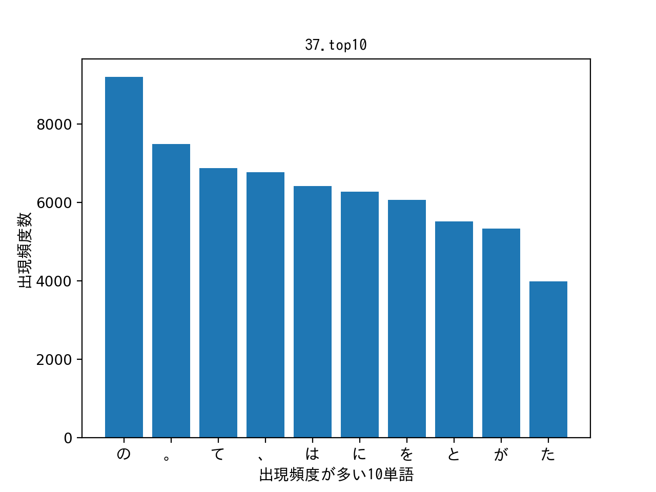
感想：pythonで初のグラフ作成でしたが、x軸やy軸に何を入れればよいかが分かればそこまで迷わずに作成できました。オプションなどのパラメータは最小限に。パラメータなどはpythonでデータサイエンスを参考にさせていただきました。日本語の表示は3分でmatplotlibを日本語対応させるを参考にさせていただきました。感謝です。

038. ヒストグラム

単語の出現頻度のヒストグラム（横軸に出現頻度，縦軸に出現頻度をとる単語の種類数を棒グラフで表したもの）を描け

histgram_graph_038.py

#-*-coding:utf-8-*-

import codecs
import ast
import collections
import operator
import matplotlib.pyplot as plt
from matplotlib.font_manager import FontProperties

if __name__ == "__main__":
    with codecs.open('neko.txt.mecab.analyze','r','utf-8') as f:
        temp_lines = f.readlines()

    temp_list=[]
    temnp_dict={}
    temp_word = ''
    for temp_line in temp_lines:
        temp_dict = ast.literal_eval(temp_line)
        temp_word = temp_dict['surface']
        temp_list.append(temp_word)

    count_dict = {}
    count_dict = collections.Counter(map(str,temp_list))

    graph_x_list =[]
    graph_y_list =[]

    for key,value in sorted(count_dict.items(),key=operator.itemgetter(1),reverse=True):
        graph_x_list.append(key)
        graph_y_list.append(value)

# 日本語の設定
    fp = FontProperties(fname=r'/Library/fonts/ipag.ttf', size=11)
# グラフのパラメータ
    plt.title("38.ヒストグラム", fontproperties=fp)
    plt.xlabel('出現頻度', fontproperties=fp)
    plt.ylabel('単語の種類数', fontproperties=fp)

#matplotlib.pyplot.bar(y=data_list, bins=binの数, range=binの最小値と最大値,normed=y軸の値で正規化する)
    plt.hist(graph_y_list,bins=20,range=(1,20),normed=True)

#グラフの表示
    plt.show()

result:

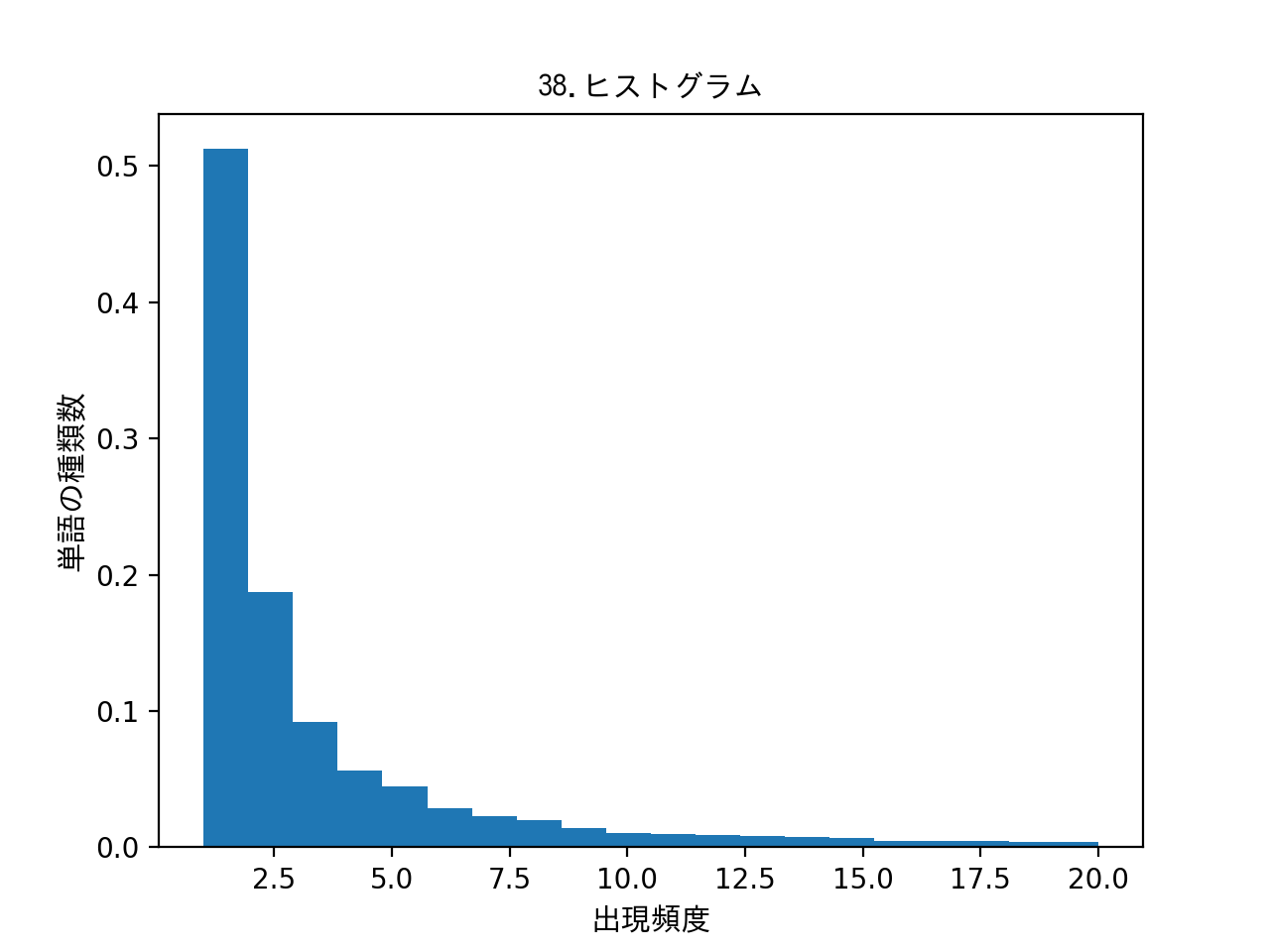
感想：スクリプトは037とほとんど同じ。差分はグラフデータをTOP10にしていない点。あとはヒストグラムのパラメータにデータを入れて作成。Y軸は単語の出現数のため、本当は正規化する必要がなかったが、試してみたかったので正規化したデータに変更。

039. Zipfの法則

単語の出現頻度順位を横軸，その出現頻度を縦軸として，両対数グラフをプロットせよ．

zipf

import codecs
import ast
import collections
import operator
import matplotlib.pyplot as plt
from matplotlib.font_manager import FontProperties

#-*-coding:utf-8-*-

if __name__ == "__main__":
    with codecs.open('neko.txt.mecab.analyze','r','utf-8') as f:
        temp_lines = f.readlines()

    temp_list = []
    temp_word = ''
    temp_dict = {}

    for temp_line in temp_lines:
        temp_dict = ast.literal_eval(temp_line)
        temp_word = temp_dict['surface']
        temp_list.append(temp_word)

    count_dict = {}
    count_dict = collections.Counter(map(str,temp_list))

    graph_x_list = []
    graph_y_list = []
    for key,value in sorted(count_dict.items(),key=operator.itemgetter(1),reverse=True):
        graph_x_list.append(key)
        graph_y_list.append(value)

#日本語の設定
    fp = FontProperties(fname=r'/Library/fonts/ipag.ttf', size=11)

#グラフのパラメータ
    plt.title("39.zipfの法則", fontproperties=fp)
    plt.xlabel('出現度順位', fontproperties=fp)
    plt.ylabel('出現頻度', fontproperties=fp)

#x/y軸を対数へ変更
    plt.xscale('log')
    plt.yscale('log')

#x軸
    x = range(1,len(graph_x_list)+1)
    y = graph_y_list

#matplotlib.pyplot.scatter(x,y=x,yはグラフに出力するデータ)
    plt.scatter(x,y)

#グラフの表示
    plt.show()

result:

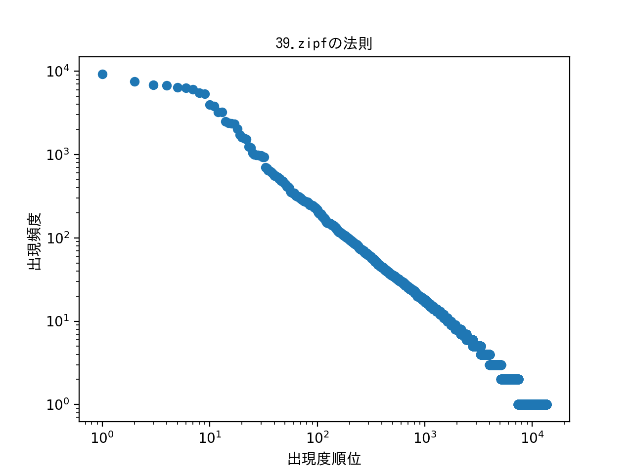
感想：法則のことはよく分からず…。素人の言語処理100本ノック:39を参考にとりあえずグラフの軸を対数へ変更したのと、X軸は単純にソートしたリストを1から数えた。Y軸には頻度のデータを入れて散布図へ入れてみた。法則のことは後で調べてみます。。。