This is an English translation of 実装技術者向けバイキュービック補間入門 その1
Introduction
Bicubic interpolation in image processing interpolates between pixels in the x and y directions using cubic functions based on the intensity values of each pixel. By computing values between pixels, you can shift an image, or scale it up or down.
Bicubic convolution algorithm
In image-processing bicubic interpolation, computing interpolation for every pixel directly is costly, so a convolution algorithm is used: precompute a convolution kernel and convolve it with each pixel of the input image. Definitions of input / interpolation functions and data sequences in the convolution algorithm are as follows.
| Name | Notation | Example | |
|---|---|---|---|
| 1 | Input function | $f(x)$ | 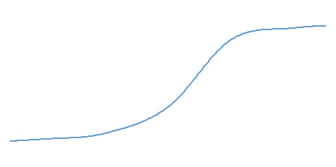 |
| 2 | Input data sequence | $f(x_j)$ | 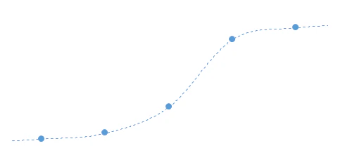 |
| 3 | Interpolation function | $g(x)$ | 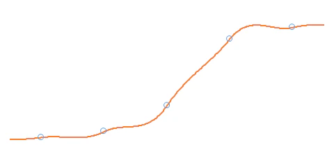 |
| 4 | Interpolated data sequence | 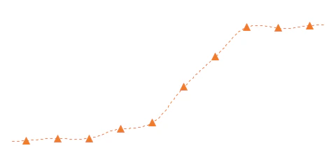 |
- Items 1 and 3 are continuous functions.
- In normal image processing, item 1 is not observable. We take item 2 and compute item 4.
- Item 2 is a sampling of item 1. Item 4 is a re-sampling of item 3. Sampling intervals are uniform, while re-sampling intervals may be arbitrary.
- The $x$ coordinate system is arbitrary.
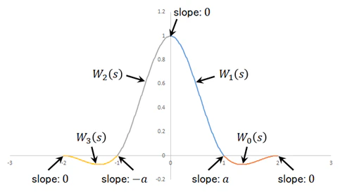
The convolution kernel is a piecewise cubic function (a composition of cubic segments) that interpolates points on a delta function (value $1$ at $s = 0$, $0$ for otherwise):
- For $1 \le s \le 2$: $W_0(s)$, passing through points $(1,0)$ and $(2,0)$
- For $0 \le s \le 1$: $W_1(s)$, passing through points $(0,1)$ and $(1,0)$
- For $-1 \le s \le 0$: $W_2(s)$, passing through points $(-1,0)$ and $(0,1)$
- For $-2 \le s \le -1$: $W_3(s)$, passing through points $(-2,0)$ and $(-1,0)$
- Otherwise: $0$
Here $s$ is the kernel coordinate:
$\quad s = (x - x_j) / h$
where $x_j$ is the nearest sampling position less than or equal to $x$, and $h$ is the sampling interval.
To make the convolution kernel smooth (first derivative continuous), add the following conditions ($a$ is a constant):
- $W_0'(s)$ (the derivative of $W_0(s)$) passes through points $(1, a)$ and $(2,0)$
- $W_1'(s)$ (the derivative of $W_1(s)$) passes through points $(0,0)$ and $(1,a)$
- $W_2'(s)$ (the derivative of $W_2(s)$) passes through points $(-1, -a)$ and $(0,0)$
- $W_3'(s)$ (the derivative of $W_3(s)$) passes through points $(-2,0)$ and $(-1, -a)$
Let $W_1(s)$ and its derivative:
$\quad W_1(s)=As^3+Bs^2+Cs+D$,
$\quad W_1'(s)=3As^2+2Bs+C$.
Substituting the boundary conditions gives the four linear equations:
$\quad W_1(0)=D=1$
$\quad W_1(1)=A+B+C+D=0$
$\quad W_1'(0)=C=0$
$\quad W_1'(1)=3A+2B+C=a$
Solving yields:
$\quad A=a+2$
$\quad B=-(a+3)$
$\quad C=0$
$\quad D=1$
So
$\quad W_1(s)=(a+2)s^3-(a+3)s^2+1$.
Similarly,
$\quad W_0(s)=as^3-5as^2+8as-4a$.
On the interval $x_j \le x \le x_{j+1}$, the interpolation function $g(x)$ is the weighted sum of the input data $f(x_{j-1}),\ f(x_j),\ f(x_{j+1}),\ f(x_{j+2})$ multiplied by the respective kernel pieces. In formula:
$\quad g(x)=W_0(s+1)\ f(x_{j-1}) + W_1(s)\ f(x_j) + W_2(s-1)\ f(x_{j+1}) + W_3(s-2)\ f(x_{j+2})$.
Since $W_2(s)$ is $W_1$ with $s$ sign-flipped and $W_3(s)$ is $W_0$ with $s$ sign-flipped:
$\quad g(x)=W_0(s+1)\ f(x_{j-1}) + W_1(s)\ f(x_j) + W_1(1-s)\ f(x_{j+1}) + W_0(2-s)\ f(x_{j+2})`$.
Computing $g(x)$ for arbitrary $x$ gives re-sampling. In image processing this is applied sequentially in $x$ and $y$ directions (order is arbitrary). If the resampling interval is constant and smaller than $h$, the image is upscaled; if larger than $h$, the image is downscaled; if equal but offset, the image is shifted. For perspective transforms or morphing the interval may vary.
Matrix notation
Transforming the convolution kernel functions yields:
$\quad W_0(s+1)=as^3-2as^2+as$
$\quad W_1(1-s)=-(a+2)s^3+(2a+3)s^2-as$
$\quad W_0(2-s)=-as^3+as^2$
Using these, the interpolation $g(x)$ in matrix form is:
g(x)=
\begin{bmatrix}
s^3 & s^2 & s & 1
\end{bmatrix}
\begin{bmatrix}
a & a+2 & -a-2 & -a \\
-2a & -a-3 & 2a+3 & a \\
a & 0 & -a & 0 \\
0 & 1 & 0 & 0
\end{bmatrix}
\begin{bmatrix}
f(x_{j-1}) \\
f(x_j) \\
f(x_{j+1}) \\
f(x_{j+2})
\end{bmatrix}
Equivalence to Catmull–Rom spline
Catmull–Rom splines are commonly known as a curve representation in design and keyframe interpolation of animation, but mathematically they are equivalent to image-processing bicubic interpolation.
A Catmull–Rom spline is a type of cubic Hermite spline. In a cubic Hermite spline, the segment between two points $\boldsymbol{p}_{k}$ and $\boldsymbol{p}_{k+1}$ is interpolated using tangent vectors $\boldsymbol{m}_{k}$ and $\boldsymbol{m}_{k+1}$ as:
$\quad \boldsymbol{p}(t) = \left(2t^3 - 3t^2 + 1\right) \boldsymbol{p}_{k} + \left(t^3 - 2t^2 + t\right) \boldsymbol{m}_{k} + \left(-2t^3 + 3t^2\right) \boldsymbol{p}_{k+1} + \left(t^3 - t^2\right) \boldsymbol{m}_{k+1}$
with $t \in [0,1]$.

By choosing the tangents as
\boldsymbol{m}_k = \frac{1}{2}(\boldsymbol{p}_{k+1} - \boldsymbol{p}_{k-1})
we obtain the Catmull–Rom spline. Substituting $\boldsymbol{m}_k = \frac{1}{2}(\boldsymbol{p}_{k+1} - \boldsymbol{p}_{k-1})$ into the cubic Hermite form and arranging in matrix form gives:
\boldsymbol{p}(t) =
\frac{1}{2}
\begin{bmatrix}
t^3 & t^2 & t & 1
\end{bmatrix}
\begin{bmatrix}
-1 & 3 & -3 & 1 \\
2 & -5 & 4 & -1 \\
-1 & 0 & 1 & 0 \\
0 & 2 & 0 & 0
\end{bmatrix}
\begin{bmatrix}
\boldsymbol{p}_{k-1} \\
\boldsymbol{p}_k \\
\boldsymbol{p}_{k+1} \\
\boldsymbol{p}_{k+2}
\end{bmatrix}
Comparing this matrix form with the bicubic interpolation matrix form above shows they agree when $a = -0.5$.
Some literature parameterizes $\frac{1}{2}$ as a tension parameter $\tau$:
\boldsymbol{m}_k = \tau (\boldsymbol{p}_{k+1} - \boldsymbol{p}_{k-1})
In that case the matrix form becomes:
\boldsymbol{p}(t) =
\begin{bmatrix}
t^3 & t^2 & t & 1
\end{bmatrix}
\begin{bmatrix}
-\tau & 2-\tau & \tau-2 & \tau \\
2\tau & \tau-3 & 3-2\tau & -\tau \\
-\tau & 0 & \tau & 0 \\
0 & 1 & 0 & 0
\end{bmatrix}
\begin{bmatrix}
\boldsymbol{p}_{k-1} \\
\boldsymbol{p}_k \\
\boldsymbol{p}_{k+1} \\
\boldsymbol{p}_{k+2}
\end{bmatrix}
Comparing this with the bicubic interpolation matrix shows equivalence when $a=-\tau$.
Single-step bicubic interpolation
In image processing bicubic interpolation is often implemented as a two-step process, applying the convolution kernel first in X then in Y. Catmull–Rom splines, however, can be extended to surfaces (bicubic patches) from the beginning. Therefore, implementing image-processing bicubic interpolation as a Catmull–Rom bicubic patch enables a single-step implementation. For hardware implementations such as FPGA or ASIC, or in some GPU pipelines, this may be a more efficient implementation.
The Catmull–Rom bicubic patch is defined as:
\boldsymbol{p}(s,t) =
\begin{bmatrix}
s^3 & s^2 & s & 1
\end{bmatrix}
\boldsymbol{M}
\begin{bmatrix}
\boldsymbol{p}_{11} & \boldsymbol{p}_{12} & \boldsymbol{p}_{13} & \boldsymbol{p}_{14} \\
\boldsymbol{p}_{21} & \boldsymbol{p}_{22} & \boldsymbol{p}_{23} & \boldsymbol{p}_{24} \\
\boldsymbol{p}_{31} & \boldsymbol{p}_{32} & \boldsymbol{p}_{33} & \boldsymbol{p}_{34} \\
\boldsymbol{p}_{41} & \boldsymbol{p}_{42} & \boldsymbol{p}_{43} & \boldsymbol{p}_{44}
\end{bmatrix}
\boldsymbol{M}^T
\begin{bmatrix}
t^3 \\
t^2 \\
t \\
1 \\
\end{bmatrix}
where
\boldsymbol{M}=
\frac{1}{2}
\begin{bmatrix}
-1 & 3 & -3 & 1 \\
2 & -5 & 4 & -1 \\
-1 & 0 & 1 & 0 \\
0 & 2 & 0 & 0
\end{bmatrix}
Using this in image-processing bicubic interpolation should allow a single-step implementation.
References
-
Robert G. Keys
Cubic convolution interpolation for digital image processing
IEEE Transactions on Acoustics, Speech, and Signal Processing Vol. ASSP-29, No.6, 1981, pp.1153-1160 -
George Wolberg
Digital Image Warping
ISBN 0-8186-8944-7, pp.129-131 -
Edwin Catmull, Raphael Rom
A class of local interpolating splines
Computer Aided Geometric Design - Proceedings of a Conference Held at The University of Utah, Salt Lake City, Utah, March 18-21, 1974
ISBN 0-12-079050-5, pp.317-326 -
Wikipedia -- Cubic Hermite spline
https://en.wikipedia.org/wiki/Cubic_Hermite_spline -
Christopher Twigg
Catmull-Rom splines
Carnegie Mellon Computer Graphics, 2003
https://www.cs.cmu.edu/~fp/courses/graphics/asst5/catmullRom.pdf
Related Posts