Introduction to Bicubic Interpolation for Implementation Engineers - #2

This is an English translation of 実装技術者向けバイキュービック補間入門　その2

Introduction

The bicubic convolution interpolation has one degree of freedom in the parameter a. Around 1972, when Rifman et al. at TRW (U.S.) first proposed it, a was fixed at $−1.0$. This was likely related to the fact that satellite images were the target. Later, in 1975, Simon of the same company suggested that $−0.5$, $−0.75$, and $−1.0$ are meaningful values. Note, however, that no remarks are made there about the interpolated results for $−0.75$ or $−1.0$. The situation is summarized in the following table.

Value of $a$	Convolution kernel	Interpolated result (interpolation function)
$-0.5$		Exact constant slope interpolation
$-0.75$	Second derivative is continuous at $x=1$
$-1.0$	Derivative at $x = 1$ matches the derivative of the sinc function

In 1981, Keys generalized the formulation and showed that only for $a = −0.5$ does the interpolation function $g(x)$ match the Taylor approximation of the input function $f(x)$ up to the second derivative (excluding the remainder term).

Keys’ proposition:

The Taylor series expansion for $f(x)$ about $x_j$ up to the second derivative at $x$ is:
$\quad f(x)=f(x_j)+shf’(x_j)+s^2h^2f’’(x_j)/2+O(h^3)$
where $O(h^3)$ denotes the remainder term.
Only in the case $a = −0.5$ does the relationship with the interpolation function $g(x)$ satisfy
$\quad f(x)-g(x)=O(h^3)$
i.e., $f(x)$ and $g(x)$ agree up to the omitted remainder term.

Despite this mathematical result favoring $−0.5$, many systems still adopt $−0.75$. The reason is unclear; a plausible guess is that interpolated images with $a = −0.75$ appear visually sharper, or that people may have mistaken "the convolution kernel’s second-derivative continuity" for "the interpolation function's second-derivative continuity". In any case, you should know which setting your processing system uses and what effects that setting causes.

Examples showing the effect of parameter "a"

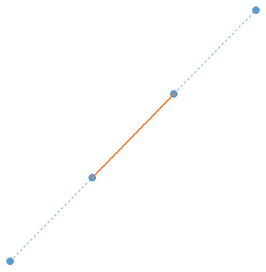
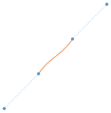
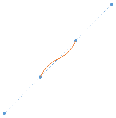
A simple illustrative case of the proposition is when $f(x)$ is a linear function. Only for $a = −0.5$ does $g(x)$ become linear (this is what "exact constant-slope interpolation" refers to). For example, with
$\quad \begin{bmatrix} f(-1) & f(0) & f(1) & f(2) \end{bmatrix} = \begin{bmatrix} -1 & 0 & 1 & 2 \end{bmatrix}$
the interpolation function on the interval $x \in [0,1]$ is
$\quad g(x) = -2(2a+1)x^3+3(2a+1)x^2-2ax$,
and only for $a = −0.5$ do the quadratic and cubic coefficients vanish so that $g(x)$ is linear.

Below are plots of this for each $a$. Blue dashed line: $f(x)$. Blue dots: sampled values of $f(x)$. Orange line: $g(x)$.

$a=-0.5$	$a=-0.75$	$a=-1.0$

Interpolation example: simple gradient image

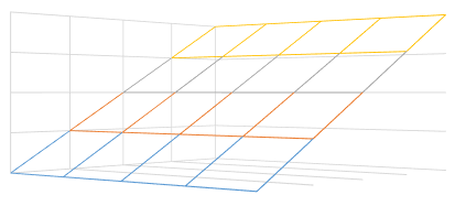
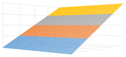
For a simple gradient image whose intensity increases monotonically only along the $x$ direction, the following shows bicubic interpolation examples. The images below are 3D plots of intensity Z for the input image and interpolated images.

Input	$a=-0.5$	$a=-0.75$	$a=-1.0$

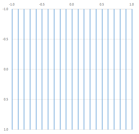
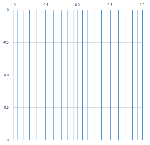
Below are contour plots of equal-intensity points.

$a=-0.5$	$a=-0.75$	$a=-1.0$

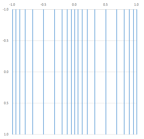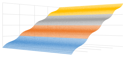
Below are examples of the simple gradient image and its 16x enlarged images. For $a = −0.75$ and $−1.0$, vertical banding artifacts (intensity nonuniformity in vertical stripes) are visible.

Input	$a=-0.5$	$a=-0.75$	$a=-1.0$	nearest-neighbor (for comparison)

Interpolation example: 45-degree gradient image

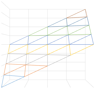
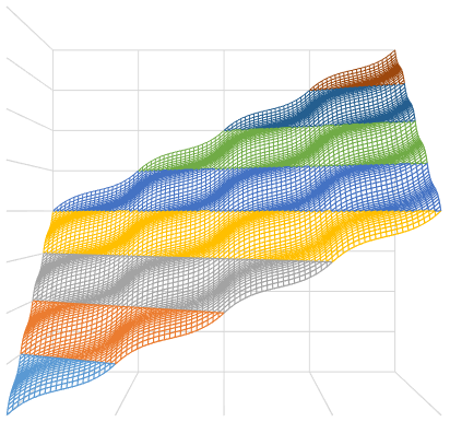
Below are 3D plots (pixel value as Z) for a 45-degree gradient image.

Input	$a=-0.5$	$a=-0.75$	$a=-1.0$

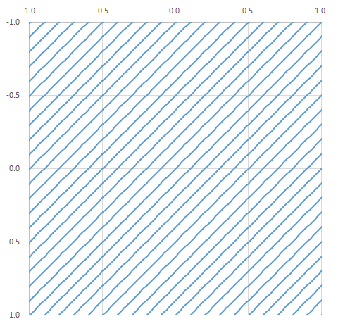
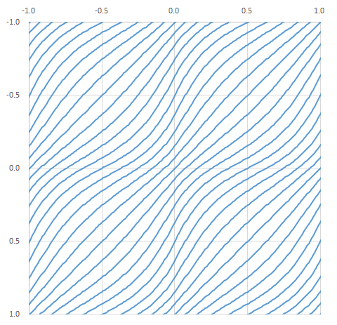
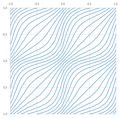
Below are contour plots of equal-intensity points.

$a=-0.5$	$a=-0.75$	$a=-1.0$

Below are the 45-degree gradient image and its 16× enlarged examples.

Input	$a=-0.5$	$a=-0.75$	$a=-1.0$	nearest-neighbor (for comparison)

Enlargement example: 45-degree stripe image

Below are a 45-degree stripe image and its 8x enlarged examples.

The 45-degree stripe image was created by drawing an anti-aliased stripe pattern at pitch $9.28\sqrt{2}$ pixels and 45 degrees using Qt's software renderer, then applying a 5x5 Gaussian via OpenCV's cv::GaussianBlur. For each setting, the enlargement examples were cropped from the 8x enlarged image at x:160, y:160, w:180, h:180.

Input	$a=-0.5$	$a=-0.75$	$a=-1.0$

Natural-image enlargement example

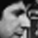
Below are enlargement examples on a natural image (a portrait) where the effect is clearly visible. For $a = −0.75$ and $−1.0$, artificial blotchy patterns appear on the temple area.

$a=-0.5$	$a=-0.75$	$a=-1.0$	nearest-neighbor (for comparison)

The above are crops (x:928, y:432, w:160, h:160) from an 8x enlargement of the following standard test image.

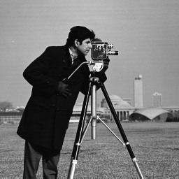
Source: MIT Works Acquired Digitally — cameraman (https://dome.mit.edu/handle/1721.3/195767)

Impact on image recognition

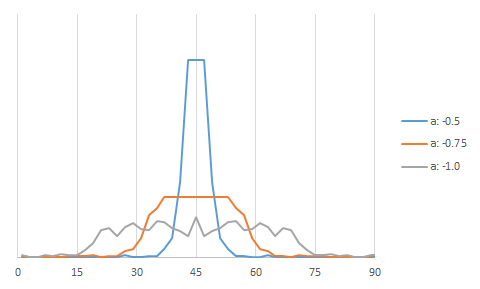
In classical pattern recognition where feature extractors are hand-designed, HOG (histogram of oriented gradients) is widely used as a feature. Below is an attempt to quantify the effect by extracting HOG from the 45-degree stripe image shown above. For $a = −0.75$ and $−1.0$, spreading of the orientation components is observed.

• HOG with 90 orientations (2-degree bins) was extracted using cv::HOGDescriptor of OpenCV.
• The entire image was treated as a single block (excluding a 20-pixel-width border).
• The histogram was normalized to sum to 1.

References

1. George Wolberg
   Digital Image Warping, pp.130-131
   ISBN 0-8186-8944-7

2. Samuel S. Rifman
   Digital rectification of ERTS multispectral imagery
   NASA Technical Report 73N28327, 1973
   https://ntrs.nasa.gov/citations/19730019595

3. K. W. Simon
   Digital Image Reconstruction and Resampling for Geometric Manipulation
   LARS Symposia, Paper 67, 1975
   https://docs.lib.purdue.edu/cgi/viewcontent.cgi?article=1068&context=lars_symp

4. Robert G Keys
   Cubic convolution interpolation for digital image processing
   IEEE Transactions on Acoustics, Speech, and Signal Processing 29 (6), 1981, pp.1153–1160
   https://ieeexplore.ieee.org/document/1163711

Related Posts