はじめに
Scikit-Learnで線形回帰をやってみます。一連の流れのコードを書いてみます。
データセット
import numpy as np
import pandas as pd
from sklearn.linear_model import LinearRegression
from sklearn.metrics import mean_squared_error, r2_score
from sklearn.model_selection import train_test_split
import matplotlib.pyplot as plt

# 1. Dataset Load

datasets = 'datasets/Boston.csv'
df = pd.read_csv(datasets)

print(f'columns: {df.columns}')
print(df.head())
print(df.describe())
結果
columns: Index(['crim', 'zn', 'indus', 'chas', 'nox', 'rm', 'age', 'dis', 'rad', 'tax',
       'ptratio', 'black', 'lstat', 'medv'],
      dtype='object')

      crim    zn  indus  chas    nox  ...  tax  ptratio   black  lstat  medv
0  0.00632  18.0   2.31     0  0.538  ...  296     15.3  396.90   4.98  24.0
1  0.02731   0.0   7.07     0  0.469  ...  242     17.8  396.90   9.14  21.6
2  0.02729   0.0   7.07     0  0.469  ...  242     17.8  392.83   4.03  34.7
3  0.03237   0.0   2.18     0  0.458  ...  222     18.7  394.63   2.94  33.4
4  0.06905   0.0   2.18     0  0.458  ...  222     18.7  396.90   5.33  36.2

             crim          zn       indus  ...       black       lstat        medv
count  506.000000  506.000000  506.000000  ...  506.000000  506.000000  506.000000
mean     3.613524   11.363636   11.136779  ...  356.674032   12.653063   22.532806
std      8.601545   23.322453    6.860353  ...   91.294864    7.141062    9.197104
min      0.006320    0.000000    0.460000  ...    0.320000    1.730000    5.000000
25%      0.082045    0.000000    5.190000  ...  375.377500    6.950000   17.025000
50%      0.256510    0.000000    9.690000  ...  391.440000   11.360000   21.200000
75%      3.677083   12.500000   18.100000  ...  396.225000   16.955000   25.000000
max     88.976200  100.000000   27.740000  ...  396.900000   37.970000   50.000000
目的変数、説明変数指定
Scikit-learnはnumpy arrayを使います。素晴らしいnumpy生態系。
したがって、Pandasのdataframeをnumpy arrayに変換します。
# 2. Dataset

target = df['medv'].to_numpy()
print(type(target))
features = df.iloc[:,:-1].to_numpy()
print(type(features))

print(target.shape)
print(features.shape)
結果
<class 'numpy.ndarray'>
<class 'numpy.ndarray'>
(506,)
(506, 13)
学習データ、テストデータ分離
# 3. Splitting the dataset into training and testing sets

X_train, X_test, y_train, y_test = train_test_split(features, target, test_size=0.2, random_state= 123)

print(X_train.shape)
print(X_test.shape)
print(y_train.shape)
print(y_test.shape)
結果
(404, 13)
(102, 13)
(404,)
(102,)
学習
# 4. Model Training

regression = LinearRegression()
model = regression.fit(X=X_train, y=y_train)
print(model.coef_)
print(model.intercept_)
結果
[-9.87931696e-02  4.75027102e-02  6.69491841e-02  1.26954150e+00
 -1.54697747e+01  4.31968412e+00 -9.80167937e-04 -1.36597953e+00
  2.84521838e-01 -1.27533606e-02 -9.13487599e-01  7.22553507e-03
 -5.43790245e-01]
31.835164121206805
評価
RMSEと決定係数R2を出します。
後、線形回帰式の重みと切片です。
# 5.Model Evaluation

y_test_predict = model.predict(X_test)
rmse = np.sqrt(mean_squared_error(y_test, y_test_predict))
r2 = r2_score(y_true=y_test, y_pred=y_test_predict)
print('The model performance for the testing set')
print(f'RMSE is {rmse}')
print(f'R2 Score is {r2}')

print(f'coefficeints are {model.coef_}')
print(f'intercept_ is {model.intercept_}')
R2スコアが0.659、モデルは悪くないですね。
結果
The model performance for the testing set
RMSE is 5.3096596650321715
R2 Score is 0.6592466510354096
coefficeints are [-9.87931696e-02  4.75027102e-02  6.69491841e-02  1.26954150e+00
 -1.54697747e+01  4.31968412e+00 -9.80167937e-04 -1.36597953e+00
  2.84521838e-01 -1.27533606e-02 -9.13487599e-01  7.22553507e-03
 -5.43790245e-01]
intercept_ is 31.835164121206805
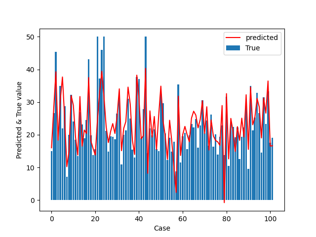
描画
True値をBarグラフで、予測値を実線で表記します。
# Plot
print(y_test.shape)
x = np.arange(0, 102 )
fig = plt.figure()
ax = fig.add_subplot(1,1,1)
ax.bar(x, y_test, label='True')
ax.plot(x,y_test_predict, color ='red', label = 'predicted')
ax.set_xlabel('Case')
ax.set_ylabel('Predicted & True value')
ax.legend()
plt.show()