More than 5 years have passed since last update.

[Keras] CIFAR10データセットで正確度75%を実現

Posted at 2020-04-01

1.はじめに

今日は、CIFAR10データセットで、正確度75%を達成する内容をご紹介します。
最初は、90%以上を目標としましたので、これからもファインチューニングを続ける予定です。

2.やりたいこと

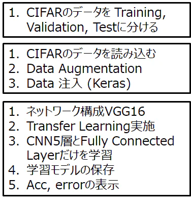
下記の図のように、普段のAIプロジェクトで行われる内容を一通り実行します。

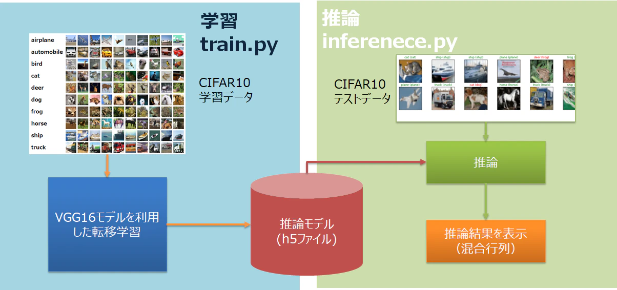
今回のタスクの特徴です。

1.　データセットはCIFAR10を利用する。データセットを(Train, Validation, Test) = (0.8, 0.1, 0.1)に分けて利用する。
2. Kerasのgeneratorを利用し、Data Augmentationを利用する。
3. 学習済みモデルVGG16を利用した、転移学習を利用する。
4. ファインチューニングされた学習モデルをh5形式で保存する。
5.　推論部では、モデルを呼び出し、テストを行う。
6.　テスト結果を混合行列(Confusion Matrix)でプロットする。
7.　学習と推論の部分を別のPythonファイルにする。

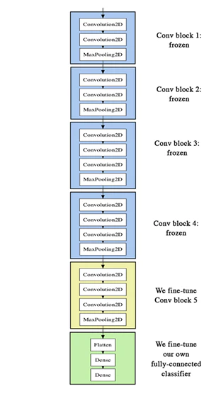
3.転移学習内容

VGG16は、五つのConv Blockと最後のFull Connected Layerで構成されています。
今回は、一つ目から四つ目のConv Blockはそのままにし、五つ目と最後のFull Connected Layerを学習することにします。

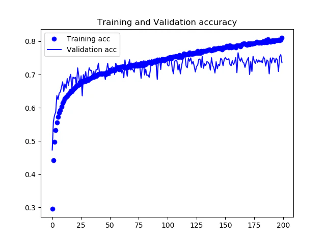
4.実行結果

4.1.学習の結果　(train.py)

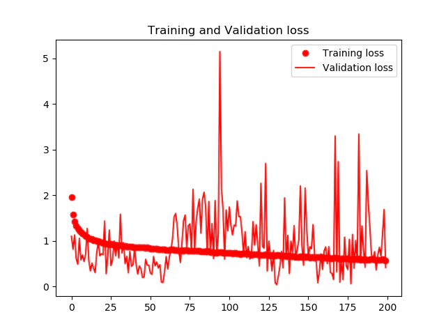
下記の図に学習時の正確度Accuracyと損失関数Lossの推移を示します。200Epochsまでの学習で、75%の正確度が得られました。
ただし、TrainデータとValidaionデータの結果が離れていくので、Overfittingが発生しているようにも見えます。

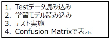
4.2.推論の結果(Inference.py)

推論の結果です。
テストデータによる正確度は平均で74.5%です。

test acc: 0.7450000047683716
Confusion Matrixの処理には、ScikitLearnのConfusion Matrixモジュールを利用しました。

5000個のテストデータの推論結果です。（5000個＝500個＊10クラス）

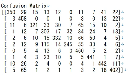
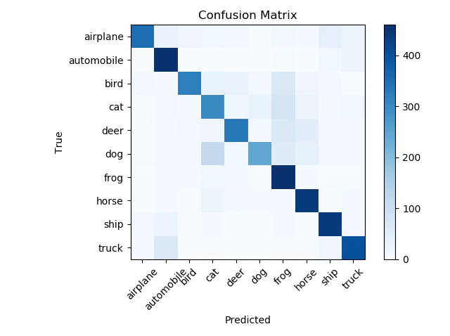
上記のテキスト形式の混同行列をMatplotlibでプロットします。

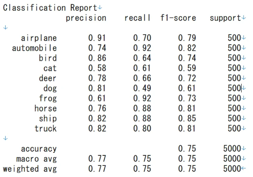
そして、各クラスごとのPrecision, Recall、F1-scoreの結果も教えてくれます。
(Precision, Recallの説明は、こちらを参考にしてください。）

5.コード

学習train.py

プログラムの構造

train.py

## Import

import os
import keras
from keras.preprocessing.image import ImageDataGenerator
from keras import models, layers
from keras.applications import VGG16
from keras import optimizers
import numpy as np
import matplotlib.pyplot as plt
from keras.callbacks import EarlyStopping




# 1.plot loss and accuracy
def plot_acc(hist):
    acc = hist.history['acc']
    val_acc = hist.history['val_acc']
    epochs = range(len(acc))
    plt.plot(epochs, acc, 'bo', label='Training acc')
    plt.plot(epochs, val_acc, 'b', label='Validation acc')
    plt.title('Training and Validation accuracy')
    plt.legend()
    pass

def plot_loss(hist):
    loss = hist.history['loss']
    val_loss = hist.history['val_loss']
    epochs = range(len(loss))
    plt.plot(epochs, loss, 'ro', label='Training loss')
    plt.plot(epochs, val_loss, 'r', label='Validation loss')
    plt.title('Training and Validation loss')
    plt.legend()


def main():

    #Initial Setting
    width_x, width_y = 32, 32
    batch_size = 32
    num_of_train_samples = 40000
    num_of_val_samples = 5000
    num_of_test_samples = 5000 #CIFAR100
    epochs = 1000


    # label_class
    classes = ['airplane', 'automobile', 'bird', 'cat', 'deer', 'dog', 'frog', 'horse', 'ship', 'truck']
    nb_classes = len(classes)

    ## 01. Data Input
    # folder information
    base_dir = 'E:\\Dataset\CIFAR10\cifar10_keras_training'
    train_data_dir = os.path.join(base_dir, 'train')
    val_data_dir = os.path.join(base_dir, 'val')
    test_data_dir = os.path.join(base_dir, 'test')

    print(train_data_dir)
    print(val_data_dir)
    print(test_data_dir)

    # Input Data Generation (with Data Augmentation)
    train_datagen = ImageDataGenerator(rescale=1. / 255,
                                       rotation_range=20,
                                       width_shift_range=0.1,
                                       height_shift_range=0.1,
                                       shear_range=0.1,
                                       zoom_range=0.1,
                                       horizontal_flip=True,
                                       fill_mode='nearest')
    val_datagen = ImageDataGenerator(rescale=1. / 255)
    test_datagen = ImageDataGenerator(rescale=1. / 255)

    train_generator = train_datagen.flow_from_directory(
        train_data_dir,
        target_size=(width_x, width_y),
        color_mode='rgb',
        classes=classes,
        class_mode='categorical',
        batch_size=batch_size,
        shuffle=False)

    val_generator = val_datagen.flow_from_directory(
        val_data_dir,
        target_size=(width_x, width_y),
        color_mode='rgb',
        classes=classes,
        class_mode='categorical',
        batch_size=batch_size,
        shuffle=False)

    test_generator = test_datagen.flow_from_directory(
        test_data_dir,
        target_size=(width_x, width_y),
        color_mode='rgb',
        classes=classes,
        class_mode='categorical',
        batch_size=batch_size,
        shuffle=False)

    ##2. CNN Model
    

    conv_base = VGG16(weights='imagenet',
                      include_top=False,
                      input_shape=(width_x, width_y, 3))
    # conv5 block fine tuning only
    conv_base.trainable = True
    set_trainable = False
    for layer in conv_base.layers:
        if layer.name == 'block5_conv1':
            set_trainable = True
        if set_trainable:
            layer.trainable = True
        else:
            layer.trainable = False

    model = models.Sequential()
    model.add(conv_base)
    model.add(layers.Flatten())
    model.add(layers.Dropout(0.5))
    model.add(layers.Dense(512, activation='relu'))
    model.add(layers.Dense(nb_classes, activation='softmax'))
    model.summary()


    model.compile(loss='categorical_crossentropy',
                  optimizer=optimizers.RMSprop(lr=1e-5),
                  metrics=['acc'])
    model.summary()

    ##3. Training
    # early_stopping = EarlyStopping(patience=20)
    history = model.fit_generator(
        train_generator,
        epochs=epochs,
        steps_per_epoch=num_of_train_samples//batch_size,
        validation_data=val_generator,
        validation_steps= num_of_val_samples//batch_size,
        verbose=2)
    # callbacks=[early_stopping]

    ##5. Model Save
    model.save('./Model/CIFAR10_trained03_seq.h5')

    ##4. Accuracy and Loss Plot
    plot_acc(history)
    plt.figure()
    plot_loss(history)
    plt.show()




## Run code

if __name__=='__main__':
    main()

推論Inference.py