はじめに
LightGBM の中身について理解するためにやってみたメモ
環境
本記事では以下を事前にインストールしておく必要がある。
- Graphviz
- Python
- numpy
- pandas
- matplotlib
- scikit-learn
- LightGBM
- RDKit
Graphvizについては、ツールをインストールした後、Pythonのライブラリをインストールする必要がある。Python: LightGBM の決定木を可視化して分岐を追ってみる や、【Windows10】Graphvizのインストール等を参考にしてほしい。
モデル構築
まずはRDKitを使ってもモデルを作成してみよう。
まずはモジュールのインポート
import numpy as np
import pandas as pd
from matplotlib import pyplot as plt
from sklearn.model_selection import train_test_split
from rdkit import rdBase, Chem
from rdkit.Chem import AllChem, Descriptors
from rdkit.ML.Descriptors import MoleculeDescriptors
import lightgbm as lgb
from lightgbm import LGBMRegressor
import graphviz
続いて、smiles列のあるcsvファイルからデータを読み込み記述子計算および、目的変数の取得を行う。
# ファイルの読み込み
import codecs
with codecs.open('../datas/raw/delaney-processed.csv', 'r', 'utf-8', 'ignore') as f:
    df = pd.read_csv(f)
# SMILESのデータを取り出す
smiles_list = df["smiles"].values

# SMILESのリストをMOLに変換
mols = []
for i, smiles in enumerate(smiles_list):
    mol = Chem.MolFromSmiles(smiles)
    if mol:
        mols.append(mol)
    else:
        print("{0} th mol is not valid".format(i))

# RDKitの記述子計算
descriptor_names = [descriptor_name[0] for descriptor_name in Descriptors._descList]
descriptor_calculator = MoleculeDescriptors.MolecularDescriptorCalculator(descriptor_names)
rdkit_descriptors_results = [descriptor_calculator.CalcDescriptors(mol) for mol in mols]
df_rdkit = pd.DataFrame(rdkit_descriptors_results, columns = descriptor_names, index=names_list)

# 目的変数の取得
df_t = df["measured log solubility in mols per litre"]
学習データとテストデータに分割しよう。
# 学習データとテストデータに分割
df_train_X, df_test_X, df_train_t, df_test_t = train_test_split(df_rdkit, df_t, test_size=0.3, random_state=0)
ここでのポイントはpandasのデータフレームの状態で分割することである。
pandasデータフレームのままLightGBMで学習を行うと可視化の際にpandasの列名が特徴名として表示されるので大変便利である。
最後に学習してモデルを構築しよう。今回は計算過程を追いやすくするため、決定木の数および深さはそれぞれ3としている。
model = LGBMRegressor(n_estimators=3, max_depth=3)
model.fit(df_train_X, df_train_t)
model.score(df_train_X, df_train_t)
スコアは低いものの、これで準備はととのった。
predictメソッドによる計算過程の確認
テストデータの1件目の化合物で予測してみよう。
model.predict([df_test_X.values[0]])
-2.89344208
と出た。勾配ブースティングの原理から、3つの決定木の計算結果の和が最終の予測結果になることは想像できる。
predictメソッドを使ってこれを確認してみよう。
ここで役に立つのが predictメソッドの start_iteration と num_iteration オプションである。
start_iteration は何番目から後の決定木を使って予測を行うかを指定する。
num_iteration はstart_iterationから数えて何個分の決定木を使って予測を行うかを指定する。
従ってstart_iteration=<決定木のインデックス>, num_iteration=1を指定することで、ぞれぞれの決定木だけを使った予測値を得ることができる。
1番目の決定木による予測結果
まずは1番目の決定によるの予測結果を求めてみよう
model.predict([df_test_X.iloc[0, :]], start_iteration=0, num_iteration=1)
-2.97228578
となる。
2番目の決定木による予測結果
つづいて2番目の決定木による予測結果を求めてみよう
model.predict([df_test_X.iloc[0, :]], start_iteration=1, num_iteration=1)
0.0604661
3番目の決定木による予測結果
最後に3番目の決定木による予測結果を求めてみよう
model.predict([df_test_X.iloc[0, :]], start_iteration=2, num_iteration=1)
0.0183776
確認
最後にこれらを和をもとめて、予測値を求めてみよう
print(-2.97228578 + 0.0604661 + 0.0183776)
-2.89344208
となり、引数なしのpredictの結果と同じ値が得られる。
決定木の可視化による計算過程の確認
予測値が複数の決定木の計算結果の和になることは分かったが、それぞれの決定木はどうなってるのかを見ていこう。
このサイト にあるようにplot_treeメソッドにより可視化することができる。
rows = 3
cols = 1
fig = plt.figure(figsize=(30, 24))
# 一本ずつプロットしていく
for i in range(rows * cols):
    ax = fig.add_subplot(rows, cols, i + 1)
    ax.set_title(f'Booster index: {i}')
    lgb.plot_tree(booster=model.booster_,
                  tree_index=i,
                  show_info='internal_value',
                  ax=ax,
                  )
plt.show()
1番目の決定木
1番目の決定木はこんな感じである。
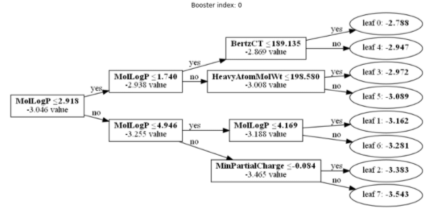
pandasのデータフレームをLightGBMの学習メソッドの引数に与えたため、図に表示される説明変数がRDKitの記述子になっていて分かりやすいと思う。
決定木に利用されている対象化合物の記述子の値は以下となっており、これを上の決定木にあてはめていくことで、predictメソッドで算出した値と同じ, -2.972 という値が得られる。
MolLogP =  1.8034
BertzCT =  59.277302439017085
HeavyAtomMolWt =  100.07599999999998
MinPartialCharge =  -0.3904614361418555
MaxPartialCharge =  0.05937549424601595
Chi4n =  0.9990707667627815
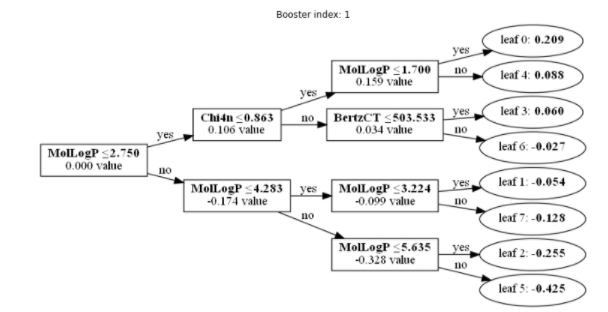
2番目の決定木
2番目の決定木は以下通りであるが、これも同様にpredictメソッドで算出した値と同じ, 0.060が得られる。
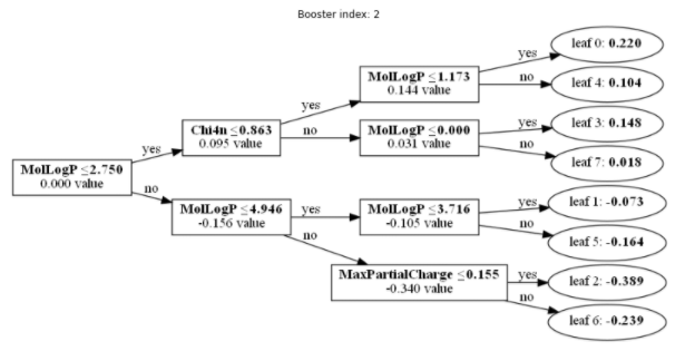
3番目の決定木
3番目の決定木は以下通りであるが、これも同様にpredictメソッドで算出した値と同じ, 0.018が得られる。
1番目~3番目の決定木の計算結果を足し合わせると最終的な予測値になることが分かる。
決定木のテキスト情報による計算過程の確認
決定木の数が何百となってくると、可視化して追っていくことは現実的ではない。
そこで、決定木の情報を解析しながら、テキストで情報を表示してみよう。
LightGBMのBoosterオブジェクトのdump_modelというメソッドを使うとjson形式でモデルの情報が得られる。
このjsonを解析することでモデル情報を得ることができる。
一例として決定木の情報をテキストで出力する関数を作ってみる。
# 決定木をテキスト情報として出力する。

# 特徴名の取得
feature_names = model.booster_.dump_model()["feature_names"]

# 決定木をルートノードから再帰的にたどり出力するメソッド
def print_tree_node(node):
    if 'split_index' in node:  # non-leaf
        print("feature = " + feature_names[node["split_feature"]] + ", threshold = " + str(node["threshold"]) + ", decision_type = " + node["decision_type"])
        print_tree_node(node['left_child'])
        print_tree_node(node['right_child'])
    else:
        print("leaf_value = " + str(node["leaf_value"]))
各項目の意味は lgb.model.dt.tree: Parse a LightGBM model json dump を参考にしてほしい。
これを使って3番目の決定木の情報を出力してみる。
tree = model.booster_.dump_model()['tree_info'][2]['tree_structure']
print_tree_node(tree)
するとルートノードから順に以下のような出力が得られ、先ほど可視化した決定木と同じ情報が得られることが分かる。
feature = MolLogP, threshold = 2.7503500000000014, decision_type = <=
feature = Chi4n, threshold = 0.8627604410602785, decision_type = <=
feature = MolLogP, threshold = 1.1729500000000004, decision_type = <=
leaf_value = 0.2197740837776413
leaf_value = 0.10397693878492793
feature = MolLogP, threshold = 1.0000000180025095e-35, decision_type = <=
leaf_value = 0.14760532911866905
leaf_value = 0.018377602562091498
feature = MolLogP, threshold = 4.946240000000005, decision_type = <=
feature = MolLogP, threshold = 3.715500000000003, decision_type = <=
leaf_value = -0.07255746476103862
leaf_value = -0.1636293624306009
feature = MaxPartialCharge, threshold = 0.15543544661242248, decision_type = <=
leaf_value = -0.3890352931889621
leaf_value = -0.2387371290297735