{biOps} 画像補間法

{biOps}のインストールについては、前記事参照の事。

サンプル画像の作成

背景は[0, 40]の一様乱数で、カクカク曲線と直線が交差しているようにする。

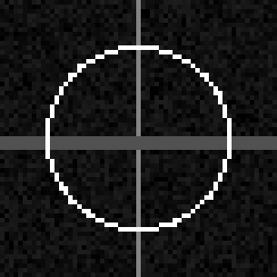
おお、それっぽい。

# 乱数のシード
set.seed(11)
# 円のxy座標を整数値で吐き出す。
x <- round(20*cos(seq(0, 2*pi, by=0.05)) + 31)
y <- round(20*sin(seq(0, 2*pi, by=0.05)) + 31)
xy <- cbind(x,y)
# 乱数に縦線と横線。
a <- matrix(runif(61*61, 0, 40), 61)
a[31,] <- 150
a[,29:31] <- 100
# ゴリ押しで円の部分を白抜き
for(i in 1:nrow(xy)){
  a[xy[i,1], xy[i,2]] <- 255
}

# 画像を保存-その1
dat <- imagedata(a)
writeTiff("sample.tiff", dat)

# 画像を保存-その2
tiff("sample.tiff", width=61, height=61)
par(mar=c(0,0,0,0))
image(1:nrow(a), 1:ncol(a), a, col=grey(0:255/255))
dev.off()

Let's 内挿

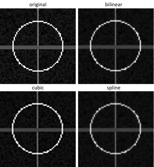
全体像

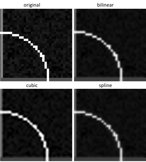
拡大像

library("biOps")

dat0 <- readTiff("sample.tiff")
dat1 <- imgScale(dat0, 3, 3, interpolation = "bilinear")
dat2 <- imgScale(dat0, 3, 3, interpolation = "cubic")
dat3 <- imgScale(dat0, 3, 3, interpolation = "spline")

writeTiff("hoge.tiff", dat)

で、何なのか。

これは、要するに、

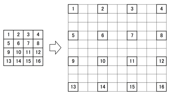
という事をして、隙間を自然に埋めよう、という事。なので、

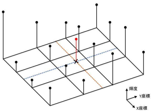
こんな事を考えて、赤い線の長さがわかれば良い。

こうですね。

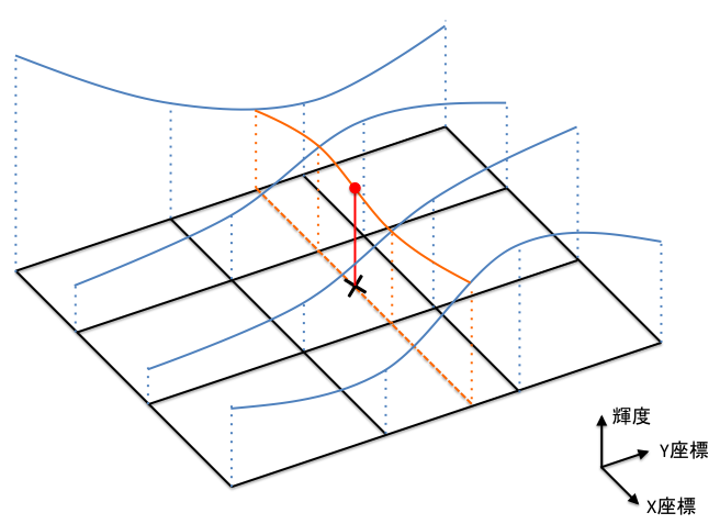
この補間関数に何を使うか、という話。

bilinerでは、近傍4点の重回帰。超シンプル。

cubicでは、近傍16点で3次関数でフィッティング。
これは、4点あれば3次関数が1義に決まるから。
一般にはbicubic法と呼ばれる。

splineでは、B-splineという関数でフィッティングする。
BはBasicのBらしい。詳しくはグーグル。

結果は見ての通り。
bicubicは結構クセがありますねぇ。
背景ノイズに強いのはB-splineでしょうか。