ガンマ分布のパラメータ指定方法まとめ

ガンマ分布

ガンマ分布は正の連続値をとる値のモデリングに使われる。
パラメータは2つあるが、ライブラリによって微妙に定義が違ったり、平均値、分散がどの程度になるか分かりづらく、いつも調べている気がするので、まとめておく。

確率密度関数

\begin{align}
f(x) &= \frac{1}{\Gamma(k) \theta^k} x^{k-1} e^{- \frac{x}{\theta}} \\
&= \frac{\lambda^k}{\Gamma(k)} x^{k-1} e^{- \lambda x}
\end{align}

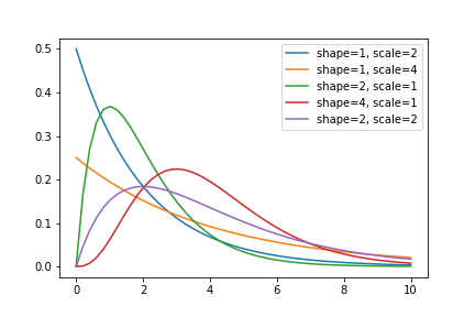
$k$: shape parameter
$\theta$: scale parameter
いずれも正の値をもつパラメータである。
ただし、ライブラリによっては、$\lambda = \frac{1}{\theta}$を使って表す場合もある。

いくつかのパラメータでプロットするとこんな感じ。

統計量

平均 $\mu= k \theta = \frac{k}{\lambda}$
分散 $v = k \theta^2 = \frac{k}{\lambda^2}$

逆に、平均、分散からパラメータを決めたい場合は、こちらを用いる。
$\theta = \frac{v}{\mu} \ (\lambda = \frac{\mu}{v})$
$k = \frac{\mu^2}{v}$

各ライブラリでのパラメータ指定方法

まとめるとこんな感じ。この表が書きたかった！

ライブラリ	shape parameter	scale parameter
numpy.random.gamma	$k$	$\theta$
scipy.stats.gamma	$a$	$\theta$
PyMC3(pm.Gamma)	$\alpha$	$1 / \beta$
TensorFlow Probability (tfp.Gamma))	concentration	1/rate
Stan (gamma)	$\alpha$	$1 / \beta$
R (rgamma)	shape	scale, 1/rate

numpy, scipyはscale parameter $\theta$ を採用しているが、PyMC3, Stan TFPなどいわゆる確率的プログラミング言語では $\theta$ の逆数での指定となっている。

$\theta$の逆数$\lambda$はrate parameterと呼ばれ、パラメータを$\alpha, \beta$と呼んでいるライブラリでは、$\lambda$による定義を採用しているようだ。

なお、PyMC3では平均（mu）, 標準偏差（sigma）でガンマ分布を指定することも可能。
また、Rではshape, rateのいずれでも指定できるようだ。

実装の確認

上記のパラメータ一覧が正しいか確認するため、各ライブラリで $Gamma(2, 2)$ から1万個の乱数を取得、確率密度関数を推定して比較してみた。

import numpy as np
import scipy as sp
import pymc3 as pm
import tensorflow_probability as tfp
import pystan
import matplotlib.pyplot as plt
import seaborn as sns

shape = 2
scale = 2
rate = 1 / scale
n_sample = 10000

xx = np.linspace(0, 20)
# ground truth
gamma_pdf = sp.stats.gamma(a=shape, scale=scale).pdf

s_np = np.random.gamma(shape=shape, scale=scale, size=n_sample)
s_sp = sp.stats.gamma(a=shape, scale=scale).rvs(size=n_sample)
s_tfp = tfp.distributions.Gamma(concentration=shape, rate=rate).sample(n_sample).numpy()
s_pm = pm.Gamma.dist(alpha=shape, beta=rate).random(size=n_sample)

fig, ax = plt.subplots()
ax.plot(xx, gamma_pdf(xx), label='truth', lw=2, c='k')
sns.kdeplot(s_np, ax=ax, label='numpy', alpha=0.8)
sns.kdeplot(s_sp, ax=ax, label='scipy', alpha=0.8)
sns.kdeplot(s_tfp, ax=ax, label='TFP', alpha=0.8)
sns.kdeplot(s_pm, ax=ax, label='PyMC3', alpha=0.8)

結果は下図の通りで、どのライブラリでも正しく実装できていることが確認できた。

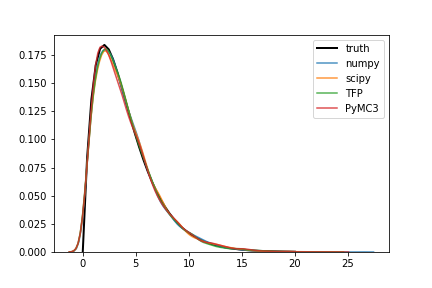
Stanだけは確率分布から直接乱数を得る方法が分からなかったので、代わりに上記で得た乱数からガンマ分布のパラメータを推定してみた。

stan_code = '''

data {
  int N;
  vector<lower=0>[N] Y;
}

parameters {
  real<lower=0> shape;
  real<lower=0> rate;
}

model {
  Y ~ gamma(shape, rate);
}

'''

data = dict(N=n_sample, Y=s_np)
stan_model = pystan.StanModel(model_code=stan_code)
fit = stan_model.sampling(data=data)
print(fit)

shape, rateパラメータの推定値はそれぞれ、1.98, 0.49となり、こちらも期待通りの結果となっている。

Inference for Stan model: anon_model_6a5d60bed963727c801dc434b96a49a1.
4 chains, each with iter=2000; warmup=1000; thin=1; 
post-warmup draws per chain=1000, total post-warmup draws=4000.

        mean se_mean     sd   2.5%    25%    50%    75%  97.5%  n_eff   Rhat
shape   1.98  8.3e-4   0.03   1.93   1.97   1.98    2.0   2.04   1016    1.0
rate    0.49  2.3e-4 7.4e-3   0.47   0.48   0.49   0.49    0.5   1020    1.0
lp__  -2.3e4    0.03   1.01 -2.3e4 -2.3e4 -2.3e4 -2.3e4 -2.3e4   1192    1.0

平均、標準偏差による分布の指定

平均、標準偏差から、該当するガンマ分布のshape, scaleを計算する関数を用意しておくと便利。

def calc_gamma_param(mu, sigma):
    return (mu / sigma)**2, sigma**2 / mu

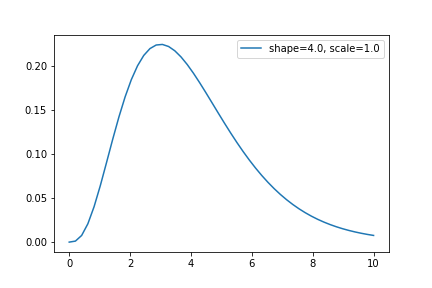
mu, sigma = 4, 2
shape, scale = calc_gamma_param(mu, sigma)

def plot_gamma(xx, shape, scale):
    plt.plot(xx, sp.stats.gamma(a=shape, scale=scale).pdf(xx), label=f'shape={shape}, scale={scale}')

xx = np.linspace(0, 10)
plot_gamma(xx, shape, scale)
plt.legend()

平均４、標準偏差２のガンマ分布。右に裾が長い分布なので、最頻値（最も確率が高い値）は平均値より小さくなることに注意。

おまけ：他の確率分布との関係

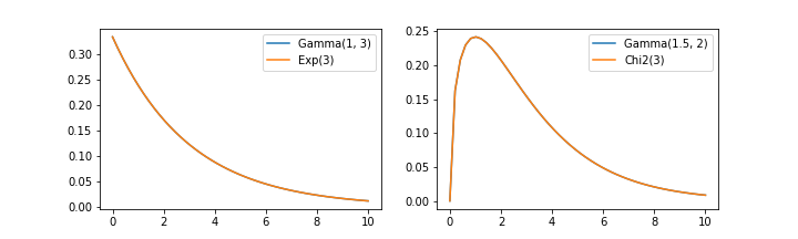
$k = 1$の時、ガンマ分布はパラメータ$\theta$の指数分布と一致する。
$k = \frac{n}{2}(n=1,2,\dots),\ \theta=2$ の時、ガンマ分布は自由度$n$のカイ二乗分布と一致する。

コードはこちら。

from scipy import stats

xx = np.linspace(0, 10)
fig, ax = plt.subplots(1, 2, figsize=(10, 3))

shape, scale = 1, 3
ax[0].plot(xx, stats.gamma(a=shape, scale=scale).pdf(xx), label=f'Gamma({shape}, {scale})')
ax[0].plot(xx, stats.expon(scale=scale).pdf(xx), label=f'Exp({scale})')
ax[0].legend()

shape, scale = 3/2, 2 
ax[1].plot(xx, stats.gamma(a=shape, scale=scale).pdf(xx), label=f'Gamma({shape}, {scale})')
ax[1].plot(xx, stats.chi2(df=2*shape).pdf(xx), label=f'Chi2({int(2*shape)})')
ax[1].legend()

plt.savefig('gamma_exp_chi2.png')