【顔分類その４】Pythonとkerasを利用した顔分類モデルの生成

目的

Pythonとkerasを利用した顔分類モデルの生成を試してみました。
学習用の水増しした画像ファイルとテスト用の画像ファイルを利用しています。

実装方法は https://blog.aidemy.net/entry/2017/12/17/214715 を参考にさせて頂きました。

サマリーはこんな感じです。

Layer (type)	Output Shape	Param #
conv2d_1 (Conv2D)	(None, 64, 64, 32)	896
max_pooling2d_1 (MaxPooling2)	(None, 32, 32, 32)	0
conv2d_2 (Conv2D)	(None, 32, 32, 32)	9248
max_pooling2d_2 (MaxPooling2)	(None, 16, 16, 32)	0
dropout_1 (Dropout)	(None, 16, 16, 32)	0
conv2d_3 (Conv2D)	(None, 16, 16, 64)	18496
max_pooling2d_3 (MaxPooling2)	(None, 8, 8, 64)	0
dropout_2 (Dropout)	(None, 8, 8, 64)	0
flatten_1 (Flatten)	(None, 4096)	0
dense_1 (Dense)	(None, 512)	2097664
dense_2 (Dense)	(None, 128)	65664
dense_3 (Dense)	(None, 2)	258

機械学習のラベルとして利用するため、2桁の0から始まる数字を画像ファイルの先頭に含めています。
結果として、0か1かの2値分類としています。

参考

【顔分類その１】PythonとGoogleカスタム検索APIを利用した画像ダウンロード
【顔分類その２】PythonとOpenCVを利用した画像ファイルからの顔の切り出し
【顔分類その３】PythonとOpenCVを利用した画像ファイルの水増し
【顔分類その４】Pythonとkerasを利用した顔分類モデルの生成
【顔分類その５】Pythonとkerasを利用して本田翼か佐倉綾音かを分類
【顔分類その６】Djangoとkerasを利用した本田翼か佐倉綾音かを分類するWebアプリ

環境

• Windows 10 x64 1809
• Python 3.6.5 x64
• Power Shell 6 x64
• Visual Studio Code x64
• Git for Windows x64
• graphviz 2.38

環境構築

• Windows 10 x64 に graphviz 2.38 をインストールします。

• 環境変数の PATH に、インストールしたgraphvizのbinフォルダを設定しておきます。

plot_modelを利用するためです。

• Windows 10 x64 に Python 3.6.x x64 をインストールします。

• 環境変数の PATH に、インストールしたPythonのフォルダとPython\Scriptsフォルダを設定しておきます。

• 下記手順で Python の仮想環境を構築し、有効化してpipをアップデートします。

> python -m venv venv
> .\venv\Scripts\activate.ps1
(venv)> python -m pip install --upgrade pip

• pip でいろいろインストールします。

(venv)> pip install pylint
(venv)> pip install opencv-python
(venv)> pip install matplotlib
(venv)> pip install tensorflow
(venv)> pip install keras
(venv)> pip install graphviz
(venv)> pip install pydotplus

graphvizに必要なpydotの代わりにpydotplusをインストールしています。

プログラム作成

• 学習モデルを生成するプログラムを Python で書きます。

• ファイル名は「img_model_gen.py」とします。

import os
import cv2
import numpy as np
import matplotlib.pyplot as plt
from keras.utils.np_utils import to_categorical
from keras.layers import Conv2D, Dense, Flatten, MaxPooling2D, Dropout
from keras.models import Sequential
# from keras.utils.vis_utils import plot_model
# tensorflowのkerasはimport時にpydot_ng,pydotplusをimportするように記述されているが，
# keras(ver=2.2.0)はimport時，pydotしかimportするようにしか記述されていないため下記とする
from tensorflow.python.keras.utils.vis_utils import plot_model

def load_images(image_directory):
    image_file_list = []
    # 指定したディレクトリ内のファイル取得
    image_file_name_list = os.listdir(image_directory)
    print(f"対象画像ファイル数：{len(image_file_name_list)}")
    for image_file_name in image_file_name_list:
        # 画像ファイルパス
        image_file_path = os.path.join(image_directory, image_file_name)
        print(f"画像ファイルパス:{image_file_path}")
        # 画像読み込み
        image = cv2.imread(image_file_path)
        if image is None:
            print(f"画像ファイル[{image_file_name}]を読み込めません")
            continue
        image_file_list.append((image_file_name, image))
    print(f"読込画像ファイル数：{len(image_file_list)}")
    return image_file_list

def labeling_images(image_file_list):
    x_data = []
    y_data = []
    for idx, (file_name, image) in enumerate(image_file_list):
        # 画像をBGR形式からRGB形式へ変換
        image = cv2.cvtColor(image, cv2.COLOR_BGR2RGB)
        # 画像配列（RGB画像）
        x_data.append(image)
        # ラベル配列（ファイル名の先頭2文字をラベルとして利用する）
        label = int(file_name[0:2])
        print(f"ラベル:{label:02}　画像ファイル名:{file_name}")
        y_data = np.append(y_data, label).reshape(idx+1, 1)
    x_data = np.array(x_data)
    print(f"ラベリング画像数：{len(x_data)}")
    return (x_data, y_data)

def delete_dir(dir_path, is_delete_top_dir=True):
    for root, dirs, files in os.walk(dir_path, topdown=False):
        for name in files:
            os.remove(os.path.join(root, name))
        for name in dirs:
            os.rmdir(os.path.join(root, name))
    if is_delete_top_dir:
        os.rmdir(dir_path)

RETURN_SUCCESS = 0
RETURN_FAILURE = -1
# Outoput Model Only
OUTPUT_MODEL_ONLY = False
# Test Image Directory
TEST_IMAGE_DIR = "./test_image"
# Train Image Directory
TRAIN_IMAGE_DIR = "./face_scratch_image"
# Output Model Directory
OUTPUT_MODEL_DIR = "./model"
# Output Model File Name
OUTPUT_MODEL_FILE = "model.h5"
# Output Plot File Name
OUTPUT_PLOT_FILE = "model.png"

def main():
    print("===================================================================")
    print("モデル学習 Keras 利用版")
    print("指定した画像ファイルをもとに学習を行いモデルを生成します。")
    print("===================================================================")

    # ディレクトリの作成
    if not os.path.isdir(OUTPUT_MODEL_DIR):
        os.mkdir(OUTPUT_MODEL_DIR)
    # ディレクトリ内のファイル削除
    delete_dir(OUTPUT_MODEL_DIR, False)

    num_classes = 2
    batch_size = 32
    epochs = 30

    # 学習用の画像ファイルの読み込み
    train_file_list = load_images(TRAIN_IMAGE_DIR)
    # 学習用の画像ファイルのラベル付け
    x_train, y_train = labeling_images(train_file_list)

    # plt.imshow(x_train[0])
    # plt.show()
    # print(y_train[0])

    # テスト用の画像ファイルの読み込み
    test_file_list = load_images(TEST_IMAGE_DIR)
    # 学習用の画像ファイルのラベル付け
    x_test, y_test = labeling_images(test_file_list)

    # plt.imshow(x_test[0])
    # plt.show()
    # print(y_test[0])

    # 画像とラベルそれぞれの次元数を確認
    print("x_train.shape:", x_train.shape)
    print("y_train.shape:", y_train.shape)
    print("x_test.shape:", x_test.shape)
    print("y_test.shape:", y_test.shape)

    # クラスラベルの1-hotベクトル化（線形分離しやすくする）
    y_train = to_categorical(y_train, num_classes)
    y_test = to_categorical(y_test, num_classes)

    # 画像とラベルそれぞれの次元数を確認
    print("x_train.shape:", x_train.shape)
    print("y_train.shape:", y_train.shape)
    print("x_test.shape:", x_test.shape)
    print("y_test.shape:", y_test.shape)

    # モデルの定義
    model = Sequential()

    # 画像に対して空間的畳み込みを行い、2次元の畳み込みレイヤーを作成する
    # 下記であれば、32通りの3×3のフィルタを用いて32通りの出力をもとに活性化関数（ReLU）を利用して特徴量（重み）を計算
    # input_shape   入力データのサイズ 64 x 64 x 3(RGB)
    # filters       フィルタ(カーネル)の数（出力数の次元）
    # kernel_size   フィルタ(カーネル)のサイズ数．3x3とか5x5とか奇数正方にすることが一般的
    # strides       ストライドの幅(フィルタを動かすピクセル数)
    # padding       データの端の取り扱い方(入力データの周囲を0で埋める(ゼロパディング)ときは'same',ゼロパディングしないときは'valid')
    # activation    活性化関数
    model.add(Conv2D(input_shape=(64, 64, 3), filters=32, kernel_size=(3, 3),
                     strides=(1, 1), padding="same", activation='relu'))
    # 2x2の4つの領域に分割して各2x2の行列の最大値をとることで出力をダウンスケールする
    # パラメータはダウンスケールする係数を決定する2つの整数のタプル
    # 各領域内の位置の違いを無視するためモデルが小さな位置変化に対して頑健（robust）となる
    model.add(MaxPooling2D(pool_size=(2, 2)))

    # 畳み込み2
    model.add(Conv2D(filters=32, kernel_size=(3, 3), strides=(1, 1),
                     padding="same", activation='relu'))
    # 出力のスケールダウン2
    model.add(MaxPooling2D(pool_size=(2, 2)))

    # ドロップアウト1
    model.add(Dropout(0.01))

    # 畳み込み3
    model.add(Conv2D(filters=64, kernel_size=(3, 3), strides=(1, 1),
                     padding="same", activation='relu'))
    # 出力のスケールダウン3
    model.add(MaxPooling2D(pool_size=(2, 2)))

    # ドロップアウト2
    model.add(Dropout(0.05))

    # 全結合層(プーリング層の出力は4次元テンソルであるため1次元のベクトルに変換)
    model.add(Flatten())

    # 予測用のレイヤー1
    model.add(Dense(512, activation='sigmoid'))

    # 予測用のレイヤー2
    model.add(Dense(128, activation='sigmoid'))

    # 予測用のレイヤー3
    model.add(Dense(num_classes, activation='softmax'))

    # コンパイル
    model.compile(optimizer='sgd',
                  loss='categorical_crossentropy',
                  metrics=['accuracy'])

    # サマリーの出力
    model.summary()

    # モデルの可視化
    plot_file_path = os.path.join(OUTPUT_MODEL_DIR, OUTPUT_PLOT_FILE)
    plot_model(model, to_file=plot_file_path, show_shapes=True)

    if OUTPUT_MODEL_ONLY:
        # 学習
        model.fit(x_train, y_train, batch_size=batch_size, epochs=epochs)
    else:
        # 学習+グラフ
        history = model.fit(x_train, y_train, batch_size=batch_size, epochs=epochs,
                            verbose=1, validation_data=(x_test, y_test))

        # 汎化精度の評価・表示
        test_loss, test_acc = model.evaluate(x_test, y_test, batch_size=batch_size, verbose=0)
        print(f"validation loss:{test_loss}\r\nvalidation accuracy:{test_acc}")

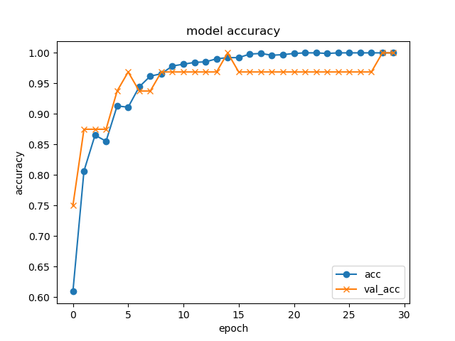
        # acc（精度）, val_acc（バリデーションデータに対する精度）のプロット
        plt.plot(history.history["acc"], label="acc", ls="-", marker="o")
        plt.plot(history.history["val_acc"], label="val_acc", ls="-", marker="x")
        plt.title('model accuracy')
        plt.xlabel("epoch")
        plt.ylabel("accuracy")
        plt.legend(loc="best")
        plt.show()

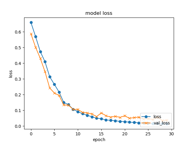
        # 損失の履歴をプロット
        plt.plot(history.history['loss'], label="loss", ls="-", marker="o")
        plt.plot(history.history['val_loss'], label="val_loss", ls="-", marker="x")
        plt.title('model loss')
        plt.xlabel('epoch')
        plt.ylabel('loss')
        plt.legend(loc='lower right')
        plt.show()

    # モデルを保存
    model_file_path = os.path.join(OUTPUT_MODEL_DIR, OUTPUT_MODEL_FILE)
    model.save(model_file_path)

    return RETURN_SUCCESS

if __name__ == "__main__":
    main()

プログラム実行

• face_scratch_imageフォルダに学習用の水増しした画像ファイルを配置します。

学習用の画像ファイルのファイル名の先頭を00か01にしておきます。

• test_imageフォルダにテスト用の画像ファイルを配置します。

テスト用の画像ファイルのファイル名の先頭を00か01にしておきます。

• プログラムを実行します。

(venv)> python .\img_model_gen.py

• epoch=30でこんな感じの結果となりました。学習にかかった時間は3分程度です。

Epoch 30/30
1024/1024 [====================] - 5s 5ms/step - loss: 0.0183 - acc: 1.0000 - val_loss: 0.0447 - val_acc: 1.0000

validation loss:0.044707685708999634
validation accuracy:1.0

最後に

深層学習で画像の分類を行いたいという勢いから、いろいろな情報を参考にやってみました。
kerasのドキュメントや様々な情報を参考に調整を行いましたが、十分な理解はできていません。
それでも、精度のグラフはおおよそ妥当なものかなと思います。
まずは試してみることを最優先としたので、じっくり学習を進めます。