2-6バックプロパゲーションを実装する
puts 'code with syntax'
import numpy as np
import tensorflow as tf
tf.reset_default_graph()
sess = tf.Session()

x_vals = np.random.normal(1, 0.1, 100)
y_vals = np.repeat(10., 100)
x_data = tf.placeholder(shape=[1], dtype=tf.float32)
y_target = tf.placeholder(shape=[1], dtype=tf.float32)

# Create variable (one model parameter = A)
A = tf.Variable(tf.random_normal(shape=[1]))

# Add operation to graph
my_output = tf.multiply(x_data, A)

# Add L2 loss operation to graph
loss = tf.square(my_output - y_target)

# Create Optimizer
my_opt = tf.train.GradientDescentOptimizer(0.02)
train_step = my_opt.minimize(loss)

# Initialize variables
init = tf.global_variables_initializer()
sess.run(init)

# Run Loop
for i in range(100):
    rand_index = np.random.choice(100)
    rand_x = [x_vals[rand_index]]
    rand_y = [y_vals[rand_index]]
    sess.run(train_step, feed_dict={x_data: rand_x, y_target: rand_y})
    if (i+1)%25==0:
        print('Step #' + str(i+1) + ' A = ' + str(sess.run(A)))
        print('Loss = ' + str(sess.run(loss, feed_dict={x_data: rand_x, y_target: rand_y})))

# Classification Example
# We will create sample data as follows:
# x-data: sample 50 random values from a normal = N(-1, 1)
#         + sample 50 random values from a normal = N(1, 1)
# target: 50 values of 0 + 50 values of 1.
#         These are essentially 100 values of the corresponding output index
# We will fit the binary classification model:
# If sigmoid(x+A) < 0.5 -> 0 else 1
# Theoretically, A should be -(mean1 + mean2)/2

tf.reset_default_graph()

# Create graph
sess = tf.Session()

# Create data
x_vals = np.concatenate((np.random.normal(-1, 1, 50), np.random.normal(3, 1, 50)))
y_vals = np.concatenate((np.repeat(0., 50), np.repeat(1., 50)))
x_data = tf.placeholder(shape=[1], dtype=tf.float32)
y_target = tf.placeholder(shape=[1], dtype=tf.float32)

# Create variable (one model parameter = A)
A = tf.Variable(tf.random_normal(mean=10, shape=[1]))

# Add operation to graph
# Want to create the operstion sigmoid(x + A)
# Note, the sigmoid() part is in the loss function
my_output = tf.add(x_data, A)

# Now we have to add another dimension to each (batch size of 1)
my_output_expanded = tf.expand_dims(my_output, 0)
y_target_expanded = tf.expand_dims(y_target, 0)

# Initialize variables
init = tf.global_variables_initializer()
sess.run(init)

# Add classification loss (cross entropy)
xentropy = tf.nn.sigmoid_cross_entropy_with_logits(logits=my_output_expanded, labels=y_target_expanded)

with tf.name_scope('summary'):
    tf.summary.scalar('loss', xentropy)
    merged = tf.summary.merge_all()
    writer = tf.summary.FileWriter('./logs', sess.graph)

# Create Optimizer
my_opt = tf.train.GradientDescentOptimizer(0.05)
train_step = my_opt.minimize(xentropy)

# Run loop
for i in range(1400):
    rand_index = np.random.choice(100)
    rand_x = [x_vals[rand_index]]
    rand_y = [y_vals[rand_index]]

    sess.run(train_step, feed_dict={x_data: rand_x, y_target: rand_y})
    if (i+1)%200==0:
        print('Step #' + str(i+1) + ' A = ' + str(sess.run(A)))
        print('Loss = ' + str(sess.run(xentropy, feed_dict={x_data: rand_x, y_target: rand_y})))

# Evaluate Predictions
predictions = []
for i in range(len(x_vals)):
    x_val = [x_vals[i]]
    prediction = sess.run(tf.round(tf.sigmoid(my_output)), feed_dict={x_data: x_val})
    predictions.append(prediction[0])

accuracy = sum(x==y for x,y in zip(predictions, y_vals))/100.
print('Ending Accuracy = ' + str(np.round(accuracy, 2)))
出力は以下のようになった。
出力
Step #25 A = [6.430147]
Loss = [8.727959]
Step #50 A = [8.748695]
Loss = [3.6893158]
Step #75 A = [9.531651]
Loss = [0.5800121]
Step #100 A = [9.720874]
Loss = [0.01573271]
Step #200 A = [4.5073967]
Loss = [[2.3545117]]
Step #400 A = [1.0466979]
Loss = [[0.00753071]]
Step #600 A = [-0.39550382]
Loss = [[0.20573217]]
Step #800 A = [-0.9899836]
Loss = [[0.05615793]]
Step #1000 A = [-0.9897802]
Loss = [[0.16368525]]
Step #1200 A = [-1.0538273]
Loss = [[0.25186038]]
Step #1400 A = [-1.132876]
Loss = [[0.07443772]]
Ending Accuracy = 0.98
コマンドターミナルに
tensorboard --logdir=./logs
を入力。するとURLが出てくるので飛ぶとTensorBoardで構造を見ることができる。
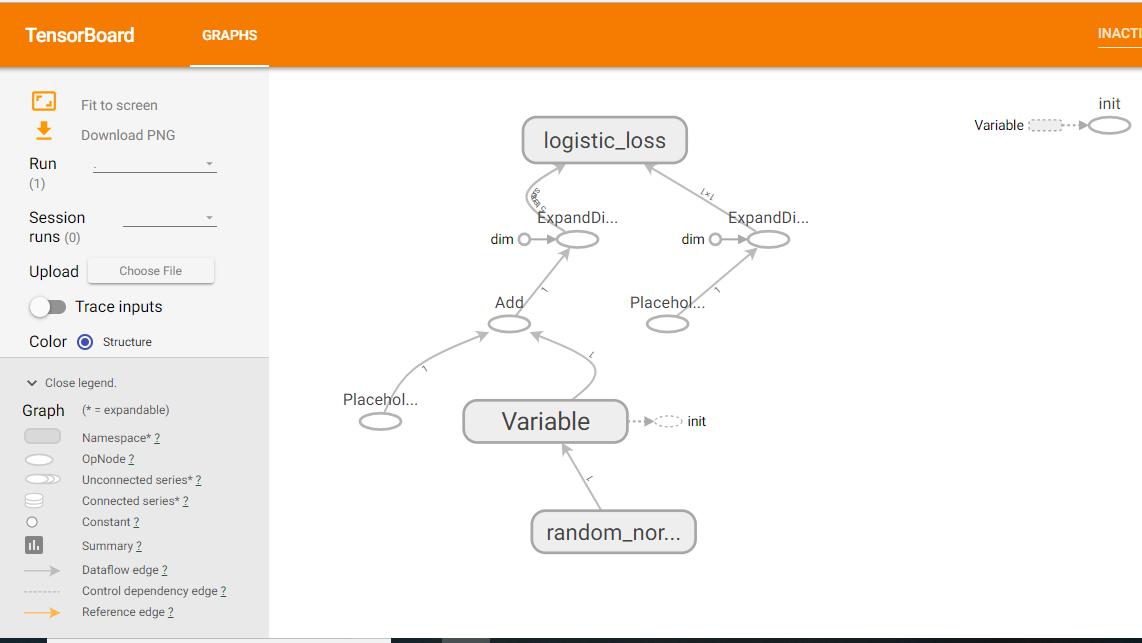
このTensorBoardを使うために
with tf.name_scope('summary'):
tf.summary.scalar('loss', xentropy)
merged = tf.summary.merge_all()
writer = tf.summary.FileWriter('./logs', sess.graph)
をコードの中に入れる。