SparkをiPython Notebook(Jupyter)で動作させ、MLlibを動かしてみるテストです。クラスタリング(KMeans)、分類:Classification(SVM, ロジスティック回帰, Random Forest)をirisデータで試しました。
環境
- OS: Mac OSX Yosemite 10.10.3
- Spark: spark-1.5.0-bin-hadoop2.6
- Python: 2.7.10 |Anaconda 2.2.0 (x86_64)| (default, May 28 2015, 17:04:42)
本稿では上記の環境で行ったものを記載していますので、他の環境では設定が異なる場合もあるかと思いますのでご注意ください。
1. Sparkバイナリのダウンロード&配置
http://spark.apache.org/downloads.html
から
spark-1.5.0-bin-hadoop2.6.tgz
をダウンロードします。(2015/9/14 現在)
ダウンロードしたバイナリを回答して適切な場所に配置します。ここでは/usr/local/bin/に置いています。
tar zxvf spark-1.5.0-bin-hadoop2.6.tar
mv spark-1.5.0-bin-hadoop2.6 /usr/local/bin/
環境変数SPARK_HOMEを.bashrcに設定します。下記を追記してください。
(初回はsource ~/.bashrcで再読み込みをして環境変数を読み込んでください。)
export SPARK_HOME=/usr/local/bin/spark-1.5.0-bin-hadoop2.6
準備ができたらiPython Notebookを起動します。
ipython notebook
1. iPython NotebookでSparkの起動
iPython Notebookで下記のコードを実行します。
import os, sys
from datetime import datetime as dt
print "loading PySpark setting..."
spark_home = os.environ.get('SPARK_HOME', None)
if not spark_home:
    raise ValueError('SPARK_HOME environment variable is not set')
sys.path.insert(0, os.path.join(spark_home, 'python'))
sys.path.insert(0, os.path.join(spark_home, 'python/lib/py4j-0.8.2.1-src.zip'))
execfile(os.path.join(spark_home, 'python/pyspark/shell.py'))
こんな表示がされれば成功です ![]()
loading PySpark setting...
/usr/local/bin/spark-1.5.0-bin-hadoop2.6
Welcome to
      ____              __
     / __/__  ___ _____/ /__
    _\ \/ _ \/ _ `/ __/  '_/
   /__ / .__/\_,_/_/ /_/\_\   version 1.5.0
      /_/

Using Python version 2.7.10 (default, May 28 2015 17:04:42)
SparkContext available as sc, HiveContext available as sqlContext.
2. MLlib(KMeans)でクラスタリング
2-1. データの準備
おなじみirisデータセットを使用します。Scikit-learnより簡単に入手できるのでこれを使います。
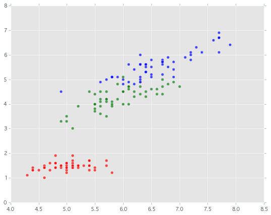
とりあえず('sepal length','petal length')の組み合わせで試します。何はともあれ散布図をプロットしてみます。
%matplotlib inline
import matplotlib.pyplot as plt
import numpy as np
import pandas as pd
from sklearn import datasets
plt.style.use('ggplot')

# http://scikit-learn.org/stable/auto_examples/datasets/plot_iris_dataset.html
iris = datasets.load_iris()
plt.figure(figsize=(9,7))

for i, color in enumerate('rgb'):
    idx = np.where(iris.target == i)[0]
    plt.scatter(iris.data[idx,0],iris.data[idx,2], c=color, s=30, alpha=.7)

plt.show()
Iris-Setosa、Iris-Versicolour、Iris-Virginicaの3種類を色分けして表示しています。
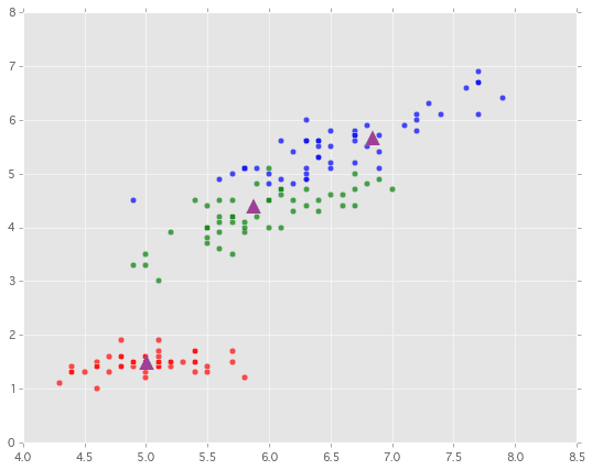
2-2 KMeansでクラスタリング
このデータから教師なし学習のクラスタリング手法の1つKMeansを試してみます。もともと3つの種別のirisですのでk=3にして正しく判定できるか試してみましょう。
# http://spark.apache.org/docs/latest/api/python/pyspark.mllib.html#module-pyspark.mllib.clustering

from pyspark.mllib.clustering import KMeans

k = 3
d_start = dt.now()

# Sparkが読み取れるようにデータを変換
data = sc.parallelize(iris.data[:,[0,2]])

# KMeansで学習実行
model = KMeans.train(data, k, initializationMode="random", seed=None)

# 結果表示
print("Final centers: " + str(model.clusterCenters))
print("Total Cost: " + str(model.computeCost(data)))
diff = dt.now() - d_start
print("{}: [end] {}".format(dt.now().strftime('%H:%M:%S'), diff ))

# ---------- Draw Graph ---------- #
plt.figure(figsize=(9,7))
for i, color in enumerate('rgb'):
    idx = np.where(iris.target == i)[0]
    plt.scatter(iris.data[idx,0],iris.data[idx,2], c=color, s=30, alpha=.7)

for i in range(k):
    plt.scatter(model.clusterCenters[i][0], model.clusterCenters[i][1], s=200, c="purple", alpha=.7, marker="^")

plt.show()
なんとなく各種類ごとの中心付近にKMeansで計算されたCenterがプロットできていますね ![]()
(KMeansの結果は初期値に依存するので、もっと変な結果となる時もあります)
Sparkを使っている部分はほんの少しだけですが、きちんと分散処理設定を行えばこれで処理が分散されます。(今回はStandaloneでのお試しなので分散されていません)
ポイントは、numpyのndarrayからsc.parallelize()でSparkのRDDに変換してそれをSparkのKMeansクラスの学習用関数train()に渡しているところです。
data = sc.parallelize(iris.data[:,[0,2]])
model = KMeans.train(data, k, initializationMode="random", seed=None)
k個のグループにクラスタリングしたそれぞれの中心点を取得するにはmodel.clusterCentersを使います。下記のコードではk=3個の中心を取得して▲マークをプロットしています。
for i in range(k):
    plt.scatter(model.clusterCenters[i][0], model.clusterCenters[i][1], s=200, c="purple", alpha=.7, marker="^")
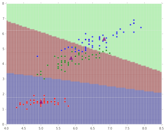
最後に座標の各点がどのようにクラスタリングされたかを可視化してみてみます。
# ------- Create Color Map ------- #
xmin = 4.0
xmax = 8.5
ymin = 0
ymax = 8
n = 100
xx = np.linspace(xmin, xmax, n)
yy = np.linspace(ymin, ymax, n)
X, Y = np.meshgrid(xx, yy)

# 2015.9.15 追加:predictの分散処理化
f_XY = np.column_stack([X.flatten(), Y.flatten()])
sc_XY = sc.parallelize(f_XY)
res = sc_XY.map(lambda data: model.predict(data))  # 学習したデータから、各点がどちらに分類されるか予測実行
Z = np.array(res.collect()).reshape(X.shape)

# 2015.9.15 削除
# Z = np.zeros_like(X)
# for i in range(n):
#    for j in range(n):
#        Z[i,j] = model.predict([xx[j],yy[i]])

# ---------- Draw Graph ---------- #
plt.figure(figsize=(9,7))
plt.xlim(xmin, xmax)
plt.ylim(ymin, ymax)

for i, color in enumerate('rgb'):
    idx = np.where(iris.target == i)[0]
    plt.scatter(iris.data[idx,0],iris.data[idx,2], c=color, s=30, alpha=.7, zorder=100)

for i in range(k):
    plt.scatter(model.clusterCenters[i][0], model.clusterCenters[i][1], s=200, c="purple", alpha=.7, marker="^", zorder=100)


plt.pcolor(X, Y, Z, alpha=0.3)
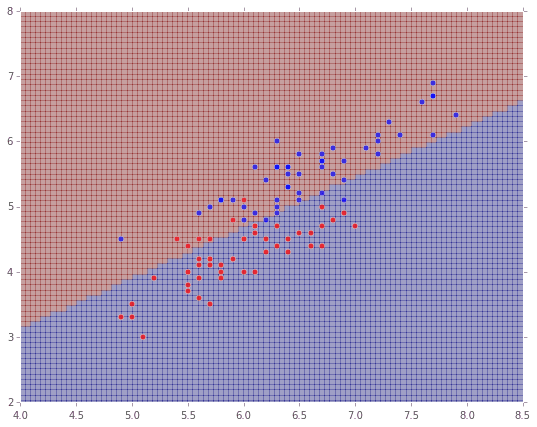
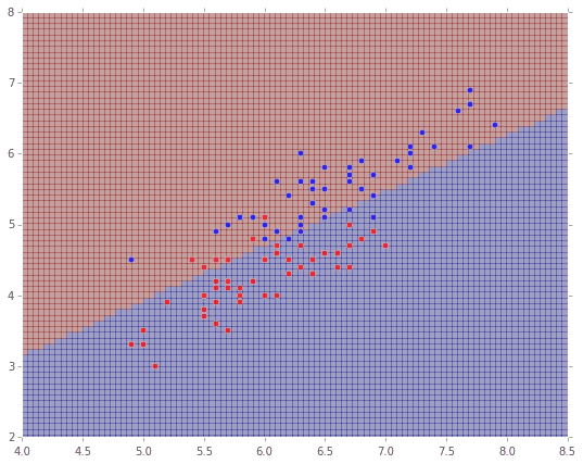
3. MLlib(SVM)でClassification
同様に今度はサポートベクターマシンです。これは2値分類なので、irisデータを2種に絞ります。
from pyspark.mllib.classification import SVMWithSGD
from pyspark.mllib.regression import LabeledPoint

# SVMは2値分類なので、2種類に絞る
idx = np.r_[ np.where(iris.target == 1)[0],  np.where(iris.target == 2)[0]]

# Sparkが読み取れるようにデータを変換
dat = np.column_stack([iris.target[idx]-1, iris.data[idx,0],iris.data[idx,2]])
data = sc.parallelize(dat)
def parsePoint(vec):
    return LabeledPoint(vec[0], vec[1:])
parsedData = data.map(parsePoint)

# SVMで学習実行
model = SVMWithSGD.train(parsedData, iterations=5000)

# ------- Predict Data ------- #
# 2015.9.15 追加:predictの分散処理化
f_XY = np.column_stack([X.flatten(), Y.flatten()])
sc_XY = sc.parallelize(f_XY)
res = sc_XY.map(lambda data: model.predict(data))  # 学習したデータから、各点がどちらに分類されるか予測実行
Z = np.array(res.collect()).reshape(X.shape)

# 2015.9.15 削除
# Z = np.zeros_like(X)
# for i in range(n):
#    for j in range(n):
#        Z[i,j] = model.predict([xx[j],yy[i]])


# ---------- Draw Graph ---------- #
plt.figure(figsize=(9,7))
xmin = 4.0
xmax = 8.5
ymin = 2
ymax = 8
plt.xlim(xmin, xmax)
plt.ylim(ymin, ymax)

# 点をプロット
for i, color in enumerate('rb'):
    idx = np.where(iris.target == i+1)[0]
    plt.scatter(iris.data[idx,0],iris.data[idx,2], c=color, s=30, alpha=.7, zorder=100)

# 塗りつぶし描画
plt.pcolor(X, Y, Z, alpha=0.3)
4. MLlib(ロジスティック回帰)でClassification
ロジスティック回帰です。こちらも2値分類ですね。
from pyspark.mllib.classification import LogisticRegressionWithLBFGS

# ロジスティック回帰で学習実行
model = LogisticRegressionWithLBFGS.train(parsedData)

# ------- Predict Data ------- #
# 2015.9.15 追加:predictの分散処理化
f_XY = np.column_stack([X.flatten(), Y.flatten()])
sc_XY = sc.parallelize(f_XY)
res = sc_XY.map(lambda data: model.predict(data))  # 学習したデータから、各点がどちらに分類されるか予測実行
Z = np.array(res.collect()).reshape(X.shape)

# 2015.9.15 削除
# Z = np.zeros_like(X)
# for i in range(n):
#    for j in range(n):
#        Z[i,j] = model.predict([xx[j],yy[i]])

# ---------- Draw Graph ---------- #
plt.figure(figsize=(9,7))
plt.xlim(xmin, xmax)
plt.ylim(ymin, ymax)

# 点をプロット
for i, color in enumerate('rb'):
    idx = np.where(iris.target == i+1)[0]
    plt.scatter(iris.data[idx,0],iris.data[idx,2], c=color, s=30, alpha=.7, zorder=100)

# 塗りつぶし描画
plt.pcolor(X, Y, Z, alpha=0.3)
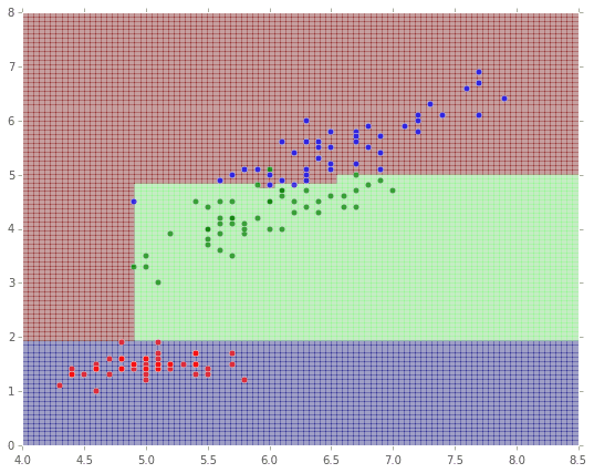
5. MLlib(ランダムフォレスト)でClassification
最後にランダムフォレストです。こちらは多値分類が可能なので、またirisの3種で分類を行います。
from pyspark.mllib.tree import RandomForest, RandomForestModel

# Sparkが読み取れるようにデータを変換
dat = np.column_stack([iris.target[:], iris.data[:,0],iris.data[:,2]])
data = sc.parallelize(dat)
parsedData = data.map(parsePoint)

# 訓練データとテストデータに分割
(trainingData, testData) = parsedData.randomSplit([0.7, 0.3])


# ランダムフォレストで学習実行
model = RandomForest.trainClassifier(trainingData, numClasses=3,
                                     categoricalFeaturesInfo={},
                                     numTrees=5, featureSubsetStrategy="auto",
                                     impurity='gini', maxDepth=4, maxBins=32)

# Evaluate model on test instances and compute test error
predictions = model.predict(testData.map(lambda x: x.features))
labelsAndPredictions = testData.map(lambda lp: lp.label).zip(predictions)
testErr = labelsAndPredictions.filter(lambda (v, p): v != p).count() / float(testData.count())
print('Test Error = ' + str(testErr))
print('Learned classification forest model:')
print(model.toDebugString())
分類結果の木構造もtoDebugString()で表示することができます。
Test Error = 0.0588235294118
Learned classification forest model:
TreeEnsembleModel classifier with 5 trees

  Tree 0:
    If (feature 1 <= 1.9)
     Predict: 0.0
    Else (feature 1 > 1.9)
     If (feature 1 <= 4.8)
      If (feature 0 <= 4.9)
       Predict: 2.0
      Else (feature 0 > 4.9)
       Predict: 1.0
     Else (feature 1 > 4.8)
      If (feature 1 <= 5.0)
       If (feature 0 <= 6.3)
        Predict: 2.0
       Else (feature 0 > 6.3)
        Predict: 1.0
      Else (feature 1 > 5.0)
       Predict: 2.0
  Tree 1:
    If (feature 1 <= 1.9)
     Predict: 0.0
    Else (feature 1 > 1.9)
     If (feature 1 <= 4.7)
      If (feature 0 <= 4.9)
       Predict: 2.0
      Else (feature 0 > 4.9)
       Predict: 1.0
     Else (feature 1 > 4.7)
      If (feature 0 <= 6.5)
       Predict: 2.0
      Else (feature 0 > 6.5)
       If (feature 1 <= 5.0)
        Predict: 1.0
       Else (feature 1 > 5.0)
        Predict: 2.0
  Tree 2:
    If (feature 1 <= 1.9)
     Predict: 0.0
    Else (feature 1 > 1.9)
     If (feature 1 <= 4.8)
      If (feature 1 <= 4.7)
       Predict: 1.0
      Else (feature 1 > 4.7)
       If (feature 0 <= 5.9)
        Predict: 1.0
       Else (feature 0 > 5.9)
        Predict: 2.0
     Else (feature 1 > 4.8)
      Predict: 2.0
  Tree 3:
    If (feature 1 <= 1.9)
     Predict: 0.0
    Else (feature 1 > 1.9)
     If (feature 1 <= 4.8)
      Predict: 1.0
     Else (feature 1 > 4.8)
      Predict: 2.0
  Tree 4:
    If (feature 1 <= 1.9)
     Predict: 0.0
    Else (feature 1 > 1.9)
     If (feature 1 <= 4.7)
      If (feature 0 <= 4.9)
       Predict: 2.0
      Else (feature 0 > 4.9)
       Predict: 1.0
     Else (feature 1 > 4.7)
      If (feature 1 <= 5.0)
       If (feature 0 <= 6.0)
        Predict: 2.0
       Else (feature 0 > 6.0)
        Predict: 1.0
      Else (feature 1 > 5.0)
       Predict: 2.0
結果を描画します。
# ------- Predict Data ------- #
Z = np.zeros_like(X)
for i in range(n):
    for j in range(n):
        Z[i,j] = model.predict([xx[j],yy[i]])

# ---------- Draw Graph ---------- #
plt.figure(figsize=(9,7))
xmin = 4.0
xmax = 8.5
ymin = 0
ymax = 8
plt.xlim(xmin, xmax)
plt.ylim(ymin, ymax)

# 点をプロット
for i, color in enumerate('rgb'):
    idx = np.where(iris.target == i)[0]
    plt.scatter(iris.data[idx,0],iris.data[idx,2], c=color, s=30, alpha=.7, zorder=100)

# 塗りつぶし描画
plt.pcolor(X, Y, Z, alpha=0.3)
次はレコメンドを扱います。
「【機械学習】Spark MLlibをPythonで動かしてレコメンデーションしてみる」
http://qiita.com/kenmatsu4/items/42fa2f17865f7914688d
修正予定
RandomForestのpredict()の並列化でエラー発生中で、対応方法模索中です。
--> どうやらこれが原因っぽい・・・。
「Spark / RDD のネストできない!」
解決できないのかな・・・。
参考
How-to: Use IPython Notebook with Apache Spark
http://blog.cloudera.com/blog/2014/08/how-to-use-ipython-notebook-with-apache-spark/
Spark 1.5.0 Machine Learning Library (MLlib) Guide
http://spark.apache.org/docs/latest/mllib-guide.html