ALDEx2 の特徴
次世代シーケンシング(NGS)は、試料から抽出されたサンプルに含まれる核酸を定量することができ、16S アンプリコン解析や、RNA-seq 解析、ChIP-seq 解析 などに利用されている。
ALDEx2 は、サンプルで検出された核酸の存在量(read 数)から、抽出元の試料に含まれる生物学的特徴量(細菌や転写産物)の組成を推定し、その組成を試料間で比較することができる解析ツールである。
NGS データの特性
上記の解析において、NGS で得られる read 数は、以下の点に留意しながら取り扱うべきである。
1) 試料から抽出された一部の核酸しか数えられていない。
NGS によって、試料中の全核酸を抽出することは不可能である。したがって、データには試料から抽出された一部の核酸しか含まれていない。また、サンプルの合計 read 数はシーケンサの性能や PCR の精度などに影響される。これらの点から、NGS データにおける read 数は、サンプル全体においてどれくらいの割合を占めるかを表す組成データに変換しなければ比較できない。
2) 多くの特徴量は試料中に微量しか存在しない。
上記の研究では、NGS で読み取られた read から、菌叢の組成や細胞の転写産物などを推定する。これらの生物学的特徴量の多くは、試料中に微量しか存在せず、サンプルによっては 1 read も読み取られないこともある。しかし、1 read も読み取られなかった特徴量が試料中には実在しているのに実在しないと推定されると、組成データの各要素が独立でないという性質上、誤った相関関係を導いてしまいやすい。
ALDEx2 では、あるサンプルにおいて 0 read の特徴量が、サンプルのばらつきによってたまたま検出されなかっただけで試料中には実在するのか、あるいは試料中にも実在しないのかを、ベイズ推定によって予測している。
ベイズ推定について
ベイズ論は、一般的な統計学で用いられる頻度論と対比して語られることが多い。では、コイントスの推定を例にして、頻度論とベイズ論を比較してみる。
頻度論では、どのような情報から確率を推定するのかを最初に決める。今回は 1000 回のコイントスの結果から、表と裏の出る確率を推定することにした。その結果、表が 499 回出て、裏が 501 回出た。この比率から表と裏が出る確率をそれぞれ推定すると 49.9%、50.1% となる。頻度論では、このように事前に指定した情報に基づいて客観的に確率を推定する。これを客観確率という。頻度論では、この後に何が起こっても(例えば裏が連続で10回出ても)客観確率を変更しない。そして、固定された客観確率をもとに、各事象が何回起こるのかという頻度(例えば3回連続で表が出る確率など)を考える。このように、確率を固定する考え方は、頻度論に基づくといえる。
| コイントス | 表 | 裏 |
|---|---|---|
| 回数 | 499回 | 501回 |
| 客観確率 | 49.9% | 50.1% |
一方でベイズ論とは、次々と新たな情報を取り入れていくことによって、確率を主観的に更新していく考え方である。ベイズ論における確率は、情報によってアップデートされていくという性質から、客観確率と対比して主観確率と呼ばれる。
では、先の試行とは別に、A 君がコイントスの結果から表と裏の出る確率を推定する場合を考える。A 君は、何回コイントスを行うかも決めずに試行を始めた。そして 2 回だけコイントスし、2 回とも表が出た。その結果から A 君は、コイントスで表が出る確率は 100% と予測した。
| コイントス | 表 | 裏 |
|---|---|---|
| 回数 | 2回 | 0回 |
| 主観確率 | 100% | 0% |
その後 A 君は、先の1000回分の試行結果を聞き、主観確率を更新した。先の試行では、表が 499 回、裏が 501 回出ていたので、自身のデータと合わせると表と裏が 501 回ずつ出たことになり、A 君は表も裏も 50% の確率で出ると判断した。
| コイントス | 表 | 裏 |
|---|---|---|
| 回数 | 501回 | 501回 |
| 主観確率 | 50% | 50% |
ベイズ推定では、更新前の主観確率を事前確率といい、更新後の主観確率を事後分布という。このように、確率を固定しない考え方は、ベイズ論に基づくといえる。
この考え方は、確率分布にも応用できる。ただしベイズ推定で取り入れられる確率分布は、確率変数を自由に変更できるように、連続型でなければならない。
ALDEx2 におけるベイズ推定【概要】
では、コイントスを用いた頻度論とベイズ論の比較を、16S アンプリコン解析の read 数に置き換えてみよう。
サンプル 1、2から、A菌、B菌、C菌に由来する read が以下のように得られたとする。
| read 数 | A菌 | B菌 | C菌 |
|---|---|---|---|
| サンプル1 | 0 | 1 | 999 |
| サンプル2 | 2 | 0 | 998 |
頻度論では、read 数の比率が、試料中で A 菌、B 菌、C 菌が最初に見つかる確率、すなわち客観確率となる。したがって、サンプル 1 の抽出元である試料 1 で A 菌が最初に見つかる確率と、サンプル 2 の抽出元である試料 2 で B 菌が最初に見つかる確率は 0% となる。
| 客観確率 | A菌 | B菌 | C菌 |
|---|---|---|---|
| 試料1 | 0% | 0.1% | 99.9% |
| 試料2 | 0.2% | 0% | 99.8% |
しかしこれらの細菌は、たまたま検出されなかっただけで、試料中には実在していた可能性もある。 頻度論では確率を変更できないため、両者を区別することができない。
そこで ALDEx2 では、どれかのサンプルで 1 read でも読み取られた特徴量は、全てのサンプルから 0.5 read が取れたと仮定する。
| read 数 | A菌 | B菌 | C菌 |
|---|---|---|---|
| サンプル1 | 0.5 | 0.5 | 0.5 |
| サンプル2 | 0.5 | 0.5 | 0.5 |
このとき事前確率は、以下のようになる。
| 事前確率 | A菌 | B菌 | C菌 |
|---|---|---|---|
| 試料1 | 33% | 33% | 33% |
| 試料2 | 33% | 33% | 33% |
ここに、実際の read 数を加算して事後確率を推定すると、
| 事後確率 | A菌 | B菌 | C菌 |
|---|---|---|---|
| 試料1 | 0.05% | 0.15% | 99.8% |
| 試料2 | 0.25% | 0.05% | 99.7% |
となる。ALDEx2 では、この事後確率にしたがってサンプリングを行い、試料中における真の存在量を推定する。このような一定の確率分布に従うサンプリングを**モンテカルロサンプリング(monte carlo sampling:MCS)**という。
ALDEx2 におけるベイズ推定【定式化】
前節の概念を定式化する。まず、以下のようにおく。なお、サンプル i は試料 i から抽出されたものとする。
- サンプル i から取れた特徴量 j の read 数:$x_{i,j}$
- 全サンプルから取れた read の種類:$m$
- 試料 i で最初に見つかる特徴量が j である確率:$µ_{i,j}$
ただし
x_i=(x_{i,1} \cdots \cdots, x_{i,m})、 µ_i=(µ_{i,1} \cdots \cdots, µ_{i,m})
とする。このとき、客観確率 $µ_{i}$ は
μ_{i} = \frac{x_i}{\sum_{j=1}^{m} x_{i,j}}
と推定される。
次に、客観確率を固定して、サンプル i から得られる特徴量 j の read 数が $X_{i,j}$ となる確率を求めてみる。ただし、
X_i=(X_{i,1} \cdots \cdots, X_{i,m})
とする。このとき、$X_i$ の確率分布は以下の多項分布になる。
Mult(X_{i}|μ_{i}) = \frac{(\sum_{j=1}^{m} X_{i,j})!}{X_{i,1}! \cdots X_{i,m}!} \prod_{j=1}^m μ_{i,j}^{X_{i,j}}
これを 尤度関数 といい、$$X_i \propto x_i$$ で最大となる。(最尤推定)
ところが尤度関数に基づく推定では、$x_{i,j}=0$ の場合、特徴量 j が試料 i に存在しないのか、試料 i に存在するがサンプル i で読み取られなかったのかを区別できない。多項分布では、サンプルの read 数に基づいて客観確率を設定しているため、試料中に存在する特徴量の真の存在量を推定することは難しい。
そこで試料 i に存在する特徴量 j の推定存在量 $α_{i,j}$ を用いて
µ^{X_{i,j}} → µ^{α_{i,j}-1}
と置き換える。この確率分布の定数項を、積分公式から求めると
Dir(µ_{i}|α_{i}) = \frac{Γ(\sum_{j=1}^{m} α_{i,j})}{Γ(α_{i,1}) \cdots Γ(α_{i,m})} \prod_{j=1}^m μ_{i,j}^{α_{i,j}-1}
となる。ただし、
α_i=(α_{i,1} \cdots \cdots, α_{i,m})
とする。この分布をディリクレ分布といい、ベイズ推定における事前分布として使用することができる。なお $α_{i,m}$ が正の整数のとき
(α_{i,j}-1)! = Γ(α_{i,j})
が成り立つ。Γ 関数は階乗を一般化したものである。
事前分布であるディリクレ分布は、尤度関数である多項分布を掛け合わせても、ディリクレ分布になる。
Dir(μ_i|α_{i}) \times Mult(X_i|μ_{i}) \propto Dir(μ_i|α_{i} + X_i)
ベイズ推定では、このような共役関係を用いて確率変数を更新している。ALDEx2では、全ての特徴量が全ての試料で微量(0.5 readに相当)に存在するという事前分布を考える。すなわち、
α_{i} = (0.5,\cdots \cdots, 0.5)
とする。また、尤度関数が最大になるように $X_i = x_i$ とおく。このような条件で事後分布
Dir(μ_i| α_i + X_i) = Dir(μ_i|(0.5,\cdots \cdots, 0.5) + (x_{i,1} \cdots \cdots, x_{i,m}))
から MCS を実施する。
組成データへの変換
試料 i の事後分布から MCS された特徴量 j の推定存在量を $V_{i,j}$ とおく。ただし、
V_i=(V_{i,1}, \cdots \cdots, V_{i,m})
とする。これを組成データ $p_i$ に変換すると、
p_{i} = (p_{i,1} \cdots \cdots, p_{i,m}) = \frac{V_i}{\sum_{j=1}^{m} V_{i,j}}
となる。組成データ $p_i$ について、サンプル i は揃えて特徴量を比較すると
p_{i,j} - p_{i,k} = \frac{V_{i,j}-V_{i,k}}{\sum_{j=1}^{m} V_{i,j}}
となる。一方で、特徴量 j を揃えてサンプルを比較すると、
p_{i,j} - p_{l,j} = \frac{V_{i,j}}{\sum_{j=1}^{m} V_{i,j}}-\frac{V_{l,j}}{\sum_{j=1}^{m} V_{l,j}}
となる。これらの比較は、MCS のやり方によって変わる擬似 read 数の合計 $\sum_{j=1}^{m} V_{l,j}$ に影響されてしまう。この影響を抑えるために、**有心対数比変換(CLR)**を用いる。
有心対数比変換(CLR)
組成データ $p_i$ に対する CLR : centered log-ratio transformation は
$$
clr(p_{i})=\left\{log_2 \frac{p_{i,1}}{g(p_i)}, log_2 \frac{p_{i,2}}{g(p_i)}, \cdots,log_2 \frac{p_{i,m}}{g(p_i)} \right\}=(c_{i,1}, \cdots \cdots, c_{i,m})=c_i
$$
である。ただし、$g(X)$ を幾何平均
$$
g(p_i)=\sqrt[n]{p_{i,1}p_{i,2}\cdots p_{i,m}}
$$
とおく。以後、$c_i$ を Dirichlet Monte-Carlo (DMC) Instance と呼ぶ。DMC Instance について、サンプル i は揃えて特徴量を比較すると
c_{i,j} - c_{i,k} = log_2 \frac{p_{i,j}}{g(p_i)}-log_2 \frac{p_{i,k}}{g(p_i)}=log_2 \frac{p_{i,j}}{p_{i,k}}
となる。一方で、特徴量 j を揃えてサンプルを比較すると、
c_{i,j} - c_{l,j} = log_2 \frac{p_{i,j}}{g(p_i)}-log_2 \frac{p_{l,j}}{g(p_i)}=log_2 \frac{p_{i,j}}{p_{l,j}}-log_2 \frac{g(p_i)}{g(p_l)}
となる。
したがって、DMC instance の比較は、サンプル間の幾何平均の差に影響される。以下、DMC instance の解析では、サンプル間の幾何平均の差が無いものと仮定している。
幾何平均の設定
ALDEx2 では、幾何平均に計算される特徴量の条件を denom という変数で指定できる。
この条件には、サンプルの read 数に基づく基準と、DMC instance に基づく基準が含まれる。
| denom | サンプルの read 数 $x_i$ | DMC instance $c_i$ |
|---|---|---|
all |
なし | なし |
iqlr |
なし | 全サンプルの分散が第一四分位数と第三四分位数の間にある。 |
lvha |
全サンプルでサンプル内の read 数が第一四分位数以上ある。 | 各群の分散がそれぞれ第一四分位数以下である。 |
zero |
各群で 1 read 以上のサンプルが最低 1 つ以上ある。 | なし |
なお、RNA-seq におけるハウスキーピング遺伝子のように、サンプル間の変動が小さいとされる特徴量を直接指定することもできる。
ALDEx2 の解析結果
ALDEx2 では、DMC instance から以下の指標が各特徴量で返される。DMC instance は、乱数に影響されるため、MCS の回数が少ないと再現性が低い。そのため、MCSの回数は 128 以上であることが推奨されている。デフォルトでは、MCS の回数は 128 に設定されており、1 つのサンプルから 128 個の DMC instance が返される。
| 指標 | 定義 | 概念 |
|---|---|---|
rab.all |
2 群の全 DMC instance における中央値 | DMC instance の大きさ |
diff.btw |
2 群間の DMC instance における差の中央値 | DMC instance の差 |
diff.win |
群内の DMC instance における差の最大値の中央値 | DMC instance の群内ばらつき |
effect |
「2 群間の DMC instance における差 ÷ 群内の DMC instance における差の最大値」の中央値 | (DMC instance の差)÷(DMC instance の群内ばらつき) |
さらに ALDEx2では、各回の DMC instances ごとに welch の t 検定が実施され、その P 値の平均値がwe.ep に返される。Benjamini-Hochberg 法によって FDR が補正された Q 値の平均値が we.eBH に返される。
例えば MCS の回数を 4回に設定すると、各回の DMC instance に対して検定が実施され、その平均値がwe.ep と we.eBH に返される。具体例を以下の表に示した。
| DMC instance | P 値 | P 値の順位 | Q 値 |
|---|---|---|---|
| 1 回目 | 0.01 | 1 位 | $0.01 \times 4/1 = 0.04$ |
| 2 回目 | 0.04 | 2 位 | $0.04 \times 4/2 = 0.10$ |
| 3 回目 | 0.08 | 3 位 | $0.08 \times 4/3 = 0.11$ |
| 4 回目 | 0.16 | 4 位 | $0.16 \times 4/4 = 0.16$ |
| Mean | 0.0725 =we.ep
|
ー | 0.1025 =we.eBH
|
一般に統計解析において帰無仮説が棄却されない場合、P 値は一様分布に従う。そのため、群間の存在率に差がない特徴量では、各回の DMC instance から得られる P 値も一様分布に従う。しかし、一様分布に従う各回の P 値の平均値である we.ep は、0.5 に収束し、偽陽性を過小評価しているという批判もある。
(出典:Thorsen, J., Brejnrod, A., Mortensen, M. et al. Large-scale benchmarking reveals false discoveries and count transformation sensitivity in 16S rRNA gene amplicon data analysis methods used in microbiome studies. Microbiome 4, 62 (2016). https://doi.org/10.1186/s40168-016-0208-8)
we.ep は、effectよりも頑健性が低いといわれている。effect>0.5 以上の特徴量は生物学的な相関関係があるとみなされる。(出典:Statistical Analysis of Microbiome Data with R (ICSA Book Series in Statistics) (英語) ペーパーバック – 2018/12/16)
R パッケージの概要
インストール
Bioconducter から ALDEx2 の R パッケージをインストールする。
if (!requireNamespace("BiocManager", quietly = TRUE))
    install.packages("BiocManager")

BiocManager::install("ALDEx2")
デモデータの取得
ALDEx2 の R パッケージには、1600 種の特徴量から構成される 14 サンプルのデモデータが収録されている。本稿では、400 種の特徴量を選び、S 群(7サンプル)と NS 群(7サンプル)を比較してみる。
library(ALDEx2)
data(selex)
dataframe  <- selex[1:400,]
conds <- c(rep("NS", 7), rep("S", 7))
set.seed(1)
ALDEx2 の解析は次のコマンドで実行できる。mc.samplesでは、MCSの回数を指定する。デフォルトでは 128 回に設定されている。これは、各サンプルから擬似サンプルを 128 回ずつ生成することを意味する。
x.all <- aldex(dataframe, conds, mc.samples=128, test="t", effect=TRUE, include.sample.summary=FALSE, denom="all", verbose=TRUE)
解析結果の保存
次のコマンドで解析結果 x.all を保存できる。
# tsv に保存
sortlist <- order(x.all$we.eBH)
x.all <- x.all[sortlist,]
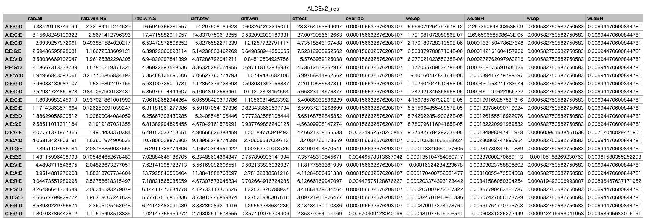
write.table(x.all,"ALDEx2_res.tsv",sep="\t",col.names=TRUE,row.names=TRUE,quote=FALSE)
# PDF に保存
pdf("ALDEx2_res.pdf")
par(mfrow=c(2,2))
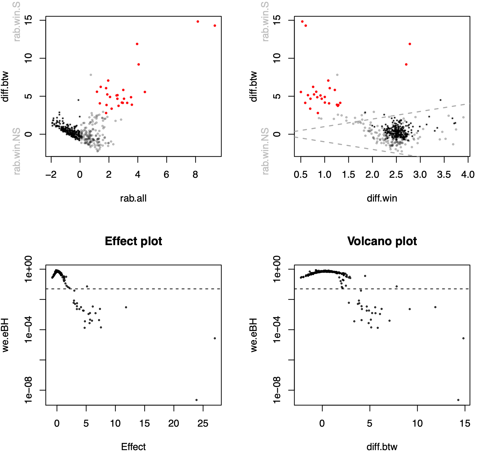
aldex.plot(x.all,type="MA",test="welch",xlab="rab.all",ylab="diff.btw",cutoff=0.05)
aldex.plot(x.all,type="MW",test="welch",xlab="diff.win",ylab="diff.btw",cutoff=0.05)
plot(x.all$effect, x.all$we.eBH, log="y", cex=0.3, col=rgb(0,0,0,1), xlab="Effect", ylab="we.eBH", main="Effect plot")
abline(h=0.05, lty=2, col="black")
plot(x.all$diff.btw, x.all$we.eBH, log="y", cex=0.3, col=rgb(0,0,0,1), xlab="diff.btw", ylab="we.eBH", main="Volcano plot")
abline(h=0.05, lty=2, col="black")
dev.off()
保存された tsv を確認してみる。各特徴量の計算結果がリストでまとめられている。
保存された PDF を確認してみる。各指標を軸にとり、各特徴量がプロットされている。
赤いプロットは、we.eBH<0.05 を満たす。
R パッケージの詳細
ここでは、ALDEx2 のソースコード から、rab.all、diff.btw、diff.win、effectの計算過程を確認する。
次のコマンドで、4 つの特徴量から構成される 14 サンプルを取得する。
14 サンプルには、NS 群に属する 7 サンプルと S 群に属する 7 サンプルが含まれる。
rm( list=ls(all=TRUE) )

data(selex)
selex <- selex[1:4,]
conds <- c(rep("NS", 7), rep("S", 7))
print(selex)
print(conds)
> rm( list=ls(all=TRUE) )
>
> data(selex)
> selex <- selex[1:4,]
> conds <- c(rep("NS", 7), rep("S", 7))
>
> print(selex)
        X1_ANS X1_BNS X1_CNS X1_DNS X2_ANS X2_CNS X2_DNS X1_AS X1_BS X1_CS X1_DS X2_AS X2_CS X2_DS
A:D:A:D    347    271    396    317    391    260    620     8     1     1     2     0     1     3
A:D:A:E    436    361    461    241    410    387    788    83     6     8    12     0     3     2
A:E:A:D    476    288    378    215    412    430    591   997  3747   662   421    37    75  6353
A:E:A:E    513    307    424    381    499    447    709 10547 12033  5394 15998   293  1816    33
> print(conds)
 [1] "NS" "NS" "NS" "NS" "NS" "NS" "NS" "S"  "S"  "S"  "S"  "S"  "S"  "S"
次に、aldex.clrという関数から、DMC instance を取得する。今回は、mc.samples=3を代入し、1 サンプルから 3 つの DMC instanceを得ることにする。
set.seed(1)
clr <- aldex.clr(selex, conds, mc.samples=3, denom="all", verbose=TRUE)
print(clr)
mc.samples<128 の場合は、警告メッセージが表示される。
> set.seed(1)
> clr <- aldex.clr(selex, conds, mc.samples=3, denom="all", verbose=TRUE)
operating in serial mode
removed rows with sums equal to zero
computing center with all features
data format is OK
dirichlet samples complete
transformation complete
 警告メッセージ:
 aldex.clr.function(reads, conds, mc.samples, denom, verbose,  で:
  values are unreliable when estimated with so few MC smps
> print(clr)
An object of class "aldex.clr"
Slot "reads":
        X1_ANS X1_BNS X1_CNS X1_DNS X2_ANS X2_CNS X2_DNS   X1_AS   X1_BS  X1_CS   X1_DS X2_AS  X2_CS  X2_DS
A:D:A:D  347.5  271.5  396.5  317.5  391.5  260.5  620.5     8.5     1.5    1.5     2.5   0.5    1.5    3.5
A:D:A:E  436.5  361.5  461.5  241.5  410.5  387.5  788.5    83.5     6.5    8.5    12.5   0.5    3.5    2.5
A:E:A:D  476.5  288.5  378.5  215.5  412.5  430.5  591.5   997.5  3747.5  662.5   421.5  37.5   75.5 6353.5
A:E:A:E  513.5  307.5  424.5  381.5  499.5  447.5  709.5 10547.5 12033.5 5394.5 15998.5 293.5 1816.5   33.5

Slot "conds":
 [1] "NS" "NS" "NS" "NS" "NS" "NS" "NS" "S"  "S"  "S"  "S"  "S"  "S"  "S"

Slot "mc.samples":
[1] 3

Slot "denom":
[1] 1 2 3 4

Slot "verbose":
[1] TRUE

Slot "useMC":
[1] FALSE

Slot "analysisData":
$X1_ANS
               [,1]        [,2]        [,3]
A:D:A:D -0.42397665 -0.45829627 -0.32611276
A:D:A:E  0.04479263  0.02637984 -0.02871167
A:E:A:D  0.16391632  0.16794445  0.11228704
A:E:A:E  0.21526769  0.26397198  0.24253738

$X1_BNS
               [,1]        [,2]        [,3]
A:D:A:D -0.18554770 -0.08490272 -0.13308168
A:D:A:E  0.16356663  0.30815560  0.31811155
A:E:A:D -0.02484904 -0.07022820 -0.14845175
A:E:A:E  0.04683011 -0.15302467 -0.03657811

$X1_CNS
               [,1]        [,2]          [,3]
A:D:A:D -0.03712156 -0.03551035 -0.0620842070
A:D:A:E  0.19236895  0.08370253  0.1385490419
A:E:A:D -0.13569723 -0.09317914 -0.0762321411
A:E:A:E -0.01955016  0.04498696 -0.0002326939

$X1_DNS
               [,1]       [,2]       [,3]
A:D:A:D  0.05561712  0.1653963  0.2024638
A:D:A:E -0.13970122 -0.1678385 -0.2587392
A:E:A:D -0.38602459 -0.4773785 -0.3518309
A:E:A:E  0.47010869  0.4798206  0.4081063

$X2_ANS
                [,1]        [,2]        [,3]
A:D:A:D -0.125133103 -0.26598644 -0.06267659
A:D:A:E -0.007141946  0.01093918 -0.07973971
A:E:A:D -0.046861771 -0.07374336 -0.03016978
A:E:A:E  0.179136820  0.32879062  0.17258607

$X2_CNS
               [,1]        [,2]        [,3]
A:D:A:D -0.49972850 -0.45804643 -0.52299509
A:D:A:E  0.05260992  0.06177432  0.09811891
A:E:A:D  0.21842910  0.14238693  0.15195193
A:E:A:E  0.22868948  0.25388518  0.27292424

$X2_DNS
               [,1]       [,2]        [,3]
A:D:A:D -0.07697430 -0.0407466 -0.06061988
A:D:A:E  0.14940322  0.2432350  0.26804343
A:E:A:D -0.15234659 -0.2771345 -0.23336928
A:E:A:E  0.07991766  0.0746461  0.02594574

$X1_AS
             [,1]      [,2]      [,3]
A:D:A:D -5.735787 -5.089553 -5.091664
A:D:A:E -1.450412 -1.649312 -2.009750
A:E:A:D  1.901454  1.653109  1.837802
A:E:A:E  5.284744  5.085755  5.263612

$X1_BS
             [,1]      [,2]      [,3]
A:D:A:D -6.548164 -7.066294 -9.026108
A:D:A:E -4.520859 -4.898072 -3.873716
A:E:A:D  4.682712  5.149446  5.599210
A:E:A:E  6.386311  6.814919  7.300614

$X1_CS
             [,1]      [,2]      [,3]
A:D:A:D -9.131040 -6.256264 -7.460525
A:D:A:E -2.556945 -3.138254 -2.156856
A:E:A:D  4.330872  3.179487  3.308641
A:E:A:E  7.357114  6.215031  6.308740

$X1_DS
             [,1]      [,2]      [,3]
A:D:A:D -4.756772 -6.104342 -5.519935
A:D:A:E -3.985074 -2.860882 -3.440124
A:E:A:D  1.730663  1.838779  1.909522
A:E:A:E  7.011183  7.126445  7.050538

$X2_AS
             [,1]      [,2]      [,3]
A:D:A:D -8.122984 -4.158034 -9.100125
A:D:A:E -3.082565 -3.520567 -1.253308
A:E:A:D  4.040404  2.312447  3.787027
A:E:A:E  7.165146  5.366155  6.566406

$X2_CS
             [,1]      [,2]       [,3]
A:D:A:D -7.555741 -3.716996 -4.0572668
A:D:A:E -2.230185 -3.412580 -2.4020789
A:E:A:D  2.724231  1.311466  0.8566282
A:E:A:E  7.061694  5.818110  5.6027174

$X2_DS
              [,1]       [,2]       [,3]
A:D:A:D -4.0097550 -4.0459283 -3.6232904
A:D:A:E -3.7638013 -3.0755179 -3.3798365
A:E:A:D  7.5097757  7.2854045  7.4368205
A:E:A:E  0.2637807 -0.1639583 -0.4336936
verbose == TRUE と設定することで、解析の進捗が返されるようにする。
verbose <- TRUE
以下、alder.effect という関数のソースコードから、rab.all、diff.btw、diff.win、effectの計算過程を確認する。
まず、clr@conds を整理する。また、特徴量の数と名前を取得する。
conditions <- clr@conds
for ( l in levels( conditions ) ) {
        levels[[l]] <- which( conditions == l )}
conditions <- as.factor( conditions )
levels     <- levels( conditions )
levels <- vector( "list", length( levels ) )
names( levels ) <- levels( conditions )
for ( l in levels( conditions ) ) {levels[[l]] <- which( conditions == l )}

nr <- numFeatures(clr)
rn <- getFeatureNames(clr)
cl2pに、全てのサンプルから 3 回ずつ得られた DMC instance を代入する。
rab <- vector( "list", 1 )
names(rab) <- c( "all")

cl2p <- NULL
for ( m in getMonteCarloInstances(clr) ) cl2p <- cbind( cl2p, m )
print(cl2p)

rab$all <- t(apply( cl2p, 1, median ))
print(rab$all)

rm(cl2p)

if (verbose == TRUE) message("rab.all  complete")
各特徴量の DMC instance は cl2p の異なる行に代入される。
各行の中央値をrab$all に返す。
> rab <- vector( "list", 1 )
> names(rab) <- c( "all")
>
> cl2p <- NULL
> for ( m in getMonteCarloInstances(clr) ) cl2p <- cbind( cl2p, m )
> print(cl2p)
               [,1]        [,2]        [,3]        [,4]        [,5]        [,6]        [,7]        [,8]          [,9]       [,10]      [,11]      [,12]        [,13]
A:D:A:D -0.42397665 -0.45829627 -0.32611276 -0.18554770 -0.08490272 -0.13308168 -0.03712156 -0.03551035 -0.0620842070  0.05561712  0.1653963  0.2024638 -0.125133103
A:D:A:E  0.04479263  0.02637984 -0.02871167  0.16356663  0.30815560  0.31811155  0.19236895  0.08370253  0.1385490419 -0.13970122 -0.1678385 -0.2587392 -0.007141946
A:E:A:D  0.16391632  0.16794445  0.11228704 -0.02484904 -0.07022820 -0.14845175 -0.13569723 -0.09317914 -0.0762321411 -0.38602459 -0.4773785 -0.3518309 -0.046861771
A:E:A:E  0.21526769  0.26397198  0.24253738  0.04683011 -0.15302467 -0.03657811 -0.01955016  0.04498696 -0.0002326939  0.47010869  0.4798206  0.4081063  0.179136820
              [,14]       [,15]       [,16]       [,17]       [,18]       [,19]      [,20]       [,21]     [,22]     [,23]     [,24]     [,25]     [,26]     [,27]
A:D:A:D -0.26598644 -0.06267659 -0.49972850 -0.45804643 -0.52299509 -0.07697430 -0.0407466 -0.06061988 -5.735787 -5.089553 -5.091664 -6.548164 -7.066294 -9.026108
A:D:A:E  0.01093918 -0.07973971  0.05260992  0.06177432  0.09811891  0.14940322  0.2432350  0.26804343 -1.450412 -1.649312 -2.009750 -4.520859 -4.898072 -3.873716
A:E:A:D -0.07374336 -0.03016978  0.21842910  0.14238693  0.15195193 -0.15234659 -0.2771345 -0.23336928  1.901454  1.653109  1.837802  4.682712  5.149446  5.599210
A:E:A:E  0.32879062  0.17258607  0.22868948  0.25388518  0.27292424  0.07991766  0.0746461  0.02594574  5.284744  5.085755  5.263612  6.386311  6.814919  7.300614
            [,28]     [,29]     [,30]     [,31]     [,32]     [,33]     [,34]     [,35]     [,36]     [,37]     [,38]      [,39]      [,40]      [,41]      [,42]
A:D:A:D -9.131040 -6.256264 -7.460525 -4.756772 -6.104342 -5.519935 -8.122984 -4.158034 -9.100125 -7.555741 -3.716996 -4.0572668 -4.0097550 -4.0459283 -3.6232904
A:D:A:E -2.556945 -3.138254 -2.156856 -3.985074 -2.860882 -3.440124 -3.082565 -3.520567 -1.253308 -2.230185 -3.412580 -2.4020789 -3.7638013 -3.0755179 -3.3798365
A:E:A:D  4.330872  3.179487  3.308641  1.730663  1.838779  1.909522  4.040404  2.312447  3.787027  2.724231  1.311466  0.8566282  7.5097757  7.2854045  7.4368205
A:E:A:E  7.357114  6.215031  6.308740  7.011183  7.126445  7.050538  7.165146  5.366155  6.566406  7.061694  5.818110  5.6027174  0.2637807 -0.1639583 -0.4336936
>
> rab$all <- t(apply( cl2p, 1, median ))
> print(rab$all)
       A:D:A:D    A:D:A:E   A:E:A:D   A:E:A:E
[1,] -2.073143 -0.7560236 0.5375287 0.3684485
>
> rm(cl2p)
>
> if (verbose == TRUE) message("rab.all  complete")
rab.all  complete
diff.btwとdiff.winの計算途中オブジェクト l2dを作成する。
ここでは、diff.winの計算途中オブジェクト l2d$win[[level]] を求める。
l2d <- vector( "list", 2 )
names( l2d ) <- c( "btw", "win" )
l2d$win <- list()

for ( level in levels(conditions) ) {
    concat <- NULL
    for ( l1 in sort( levels[[level]] ) ) {
        concat <- cbind(  getMonteCarloReplicate(clr,l1),concat )

    }

    print('concat')

    print(concat)

    if ( ncol(concat) < 10000 ){
        sampl1 <- t(apply(concat, 1, function(x){sample(x, ncol(concat))}))
        sampl2 <- t(apply(concat, 1, function(x){sample(x, ncol(concat))}))
    } else {
        sampl1 <- t(apply(concat, 1, function(x){sample(x, 10000)}))
        sampl2 <- t(apply(concat, 1, function(x){sample(x, 10000)}))
    }

    print('sampl1')
    print(sampl1)
    print('sampl2')
    print(sampl2)

    l2d$win[[level]] <- cbind( l2d$win[[level]] , abs( sampl1 - sampl2 ) )

    print(level)

    print('l2d$win[[level]] ')

    print(l2d$win[[level]])

    rm(sampl1)
    rm(sampl2)
}
if (verbose == TRUE) message("within sample difference calculated")
群内の DMC instance から構成される concat を並び替えたsampl1とsampl2の各成分の差を、NS 群と S 群のそれぞれで計算し、 l2d$win[["NS"]]とl2d$win[["S"]]に返す。
差は最大で 10000 個までしか返さない。
> l2d <- vector( "list", 2 )
> names( l2d ) <- c( "btw", "win" )
> l2d$win <- list()
>
> for ( level in levels(conditions) ) {
+     concat <- NULL
+     for ( l1 in sort( levels[[level]] ) ) {
+         concat <- cbind(  getMonteCarloReplicate(clr,l1),concat )
+
+     }
+
+     print('concat')
+
+     print(concat)
+
+     if ( ncol(concat) < 10000 ){
+         sampl1 <- t(apply(concat, 1, function(x){sample(x, ncol(concat))}))
+         sampl2 <- t(apply(concat, 1, function(x){sample(x, ncol(concat))}))
+     } else {
+         sampl1 <- t(apply(concat, 1, function(x){sample(x, 10000)}))
+         sampl2 <- t(apply(concat, 1, function(x){sample(x, 10000)}))
+     }
+
+     print('sampl1')
+     print(sampl1)
+     print('sampl2')
+     print(sampl2)
+
+     l2d$win[[level]] <- cbind( l2d$win[[level]] , abs( sampl1 - sampl2 ) )
+
+     print(level)
+
+     print('l2d$win[[level]] ')
+
+     print(l2d$win[[level]])
+
+     rm(sampl1)
+     rm(sampl2)
+ }
[1] "concat"
               [,1]       [,2]        [,3]        [,4]        [,5]        [,6]         [,7]        [,8]        [,9]       [,10]      [,11]      [,12]       [,13]
A:D:A:D -0.07697430 -0.0407466 -0.06061988 -0.49972850 -0.45804643 -0.52299509 -0.125133103 -0.26598644 -0.06267659  0.05561712  0.1653963  0.2024638 -0.03712156
A:D:A:E  0.14940322  0.2432350  0.26804343  0.05260992  0.06177432  0.09811891 -0.007141946  0.01093918 -0.07973971 -0.13970122 -0.1678385 -0.2587392  0.19236895
A:E:A:D -0.15234659 -0.2771345 -0.23336928  0.21842910  0.14238693  0.15195193 -0.046861771 -0.07374336 -0.03016978 -0.38602459 -0.4773785 -0.3518309 -0.13569723
A:E:A:E  0.07991766  0.0746461  0.02594574  0.22868948  0.25388518  0.27292424  0.179136820  0.32879062  0.17258607  0.47010869  0.4798206  0.4081063 -0.01955016
              [,14]         [,15]       [,16]       [,17]       [,18]       [,19]       [,20]       [,21]
A:D:A:D -0.03551035 -0.0620842070 -0.18554770 -0.08490272 -0.13308168 -0.42397665 -0.45829627 -0.32611276
A:D:A:E  0.08370253  0.1385490419  0.16356663  0.30815560  0.31811155  0.04479263  0.02637984 -0.02871167
A:E:A:D -0.09317914 -0.0762321411 -0.02484904 -0.07022820 -0.14845175  0.16391632  0.16794445  0.11228704
A:E:A:E  0.04498696 -0.0002326939  0.04683011 -0.15302467 -0.03657811  0.21526769  0.26397198  0.24253738
[1] "sampl1"
                 [,1]        [,2]        [,3]        [,4]        [,5]        [,6]        [,7]        [,8]        [,9]       [,10]       [,11]      [,12]       [,13]
A:D:A:D -0.0769742974 -0.06061988  0.16539634 -0.03712156 -0.45804643  0.20246378  0.05561712 -0.06208421 -0.26598644 -0.04074660 -0.49972850 -0.1330817 -0.06267659
A:D:A:E  0.0109391847  0.26804343  0.04479263  0.14940322  0.05260992  0.19236895 -0.25873918  0.31811155 -0.02871167  0.06177432  0.13854904 -0.1397012  0.02637984
A:E:A:D -0.2333692791  0.16794445 -0.03016978 -0.35183091 -0.14845175 -0.04686177 -0.13569723 -0.47737845  0.21842910  0.11228704 -0.02484904 -0.1523466  0.14238693
A:E:A:E -0.0002326939  0.21526769  0.25388518  0.04498696  0.17913682  0.04683011  0.47982060  0.24253738  0.47010869 -0.01955016  0.07464610  0.2729242 -0.03657811
              [,14]        [,15]      [,16]       [,17]       [,18]      [,19]       [,20]      [,21]
A:D:A:D -0.52299509 -0.326112757 -0.1251331 -0.08490272 -0.18554770 -0.4239766 -0.03551035 -0.4582963
A:D:A:E  0.08370253 -0.007141946 -0.1678385  0.09811891 -0.07973971  0.1635666  0.30815560  0.2432350
A:E:A:D -0.07022820 -0.093179138  0.1639163 -0.07623214 -0.38602459  0.1519519 -0.07374336 -0.2771345
A:E:A:E  0.26397198  0.079917663 -0.1530247  0.32879062  0.17258607  0.4081063  0.02594574  0.2286895
[1] "sampl2"
               [,1]        [,2]        [,3]        [,4]        [,5]        [,6]        [,7]       [,8]        [,9]      [,10]       [,11]       [,12]       [,13]
A:D:A:D -0.26598644 -0.04074660 -0.06267659 -0.32611276 -0.03551035  0.05561712 -0.49972850 -0.4580464 -0.18554770  0.2024638 -0.06208421 -0.12513310 -0.13308168
A:D:A:E  0.06177432  0.01093918  0.19236895  0.05260992 -0.13970122  0.09811891 -0.16783849  0.2432350 -0.02871167  0.3181115  0.14940322  0.16356663  0.02637984
A:E:A:D -0.07374336  0.16794445  0.16391632  0.14238693 -0.27713453 -0.14845175 -0.02484904 -0.3518309 -0.23336928 -0.3860246 -0.07022820 -0.04686177  0.11228704
A:E:A:E -0.15302467  0.47982060  0.17258607  0.32879062 -0.01955016  0.27292424  0.02594574  0.2639720  0.40810631  0.4701087  0.07991766  0.04683011  0.04498696
              [,14]       [,15]       [,16]       [,17]        [,18]         [,19]       [,20]       [,21]
A:D:A:D -0.03712156 -0.08490272 -0.45829627 -0.07697430  0.165396340 -0.4239766451 -0.52299509 -0.06061988
A:D:A:E  0.13854904  0.26804343 -0.25873918 -0.07973971 -0.007141946  0.0837025343  0.30815560  0.04479263
A:E:A:D -0.47737845  0.15195193 -0.03016978 -0.07623214  0.218429095 -0.1356972267 -0.09317914 -0.15234659
A:E:A:E  0.22868948  0.25388518  0.24253738  0.07464610  0.179136820 -0.0002326939 -0.03657811  0.21526769
[1] "NS"
[1] "l2d$win[[level]] "
              [,1]       [,2]       [,3]      [,4]      [,5]       [,6]      [,7]       [,8]       [,9]     [,10]       [,11]       [,12]      [,13]      [,14]     [,15]
A:D:A:D 0.18901214 0.01987328 0.22807293 0.2889912 0.4225361 0.14684666 0.5553456 0.39596222 0.08043873 0.2432104 0.437644294 0.007948578 0.07040509 0.48587353 0.2412100
A:D:A:E 0.05083513 0.25710424 0.14757632 0.0967933 0.1923111 0.09425004 0.0909007 0.07487651 0.00000000 0.2563372 0.010854182 0.303267850 0.00000000 0.05484651 0.2751854
A:E:A:D 0.15962591 0.00000000 0.19408610 0.4942178 0.1286828 0.10158998 0.1108482 0.12554755 0.45179837 0.4983116 0.045379162 0.105484819 0.03009989 0.40715025 0.2451311
A:E:A:E 0.15279198 0.26455291 0.08129911 0.2838037 0.1986870 0.22609413 0.4538749 0.02143460 0.06200238 0.4896589 0.005271564 0.226094133 0.08156507 0.03528250 0.1739675
            [,16]       [,17]       [,18]     [,19]      [,20]      [,21]
A:D:A:D 0.3331632 0.007928424 0.350944042 0.0000000 0.48748474 0.39767639
A:D:A:E 0.0909007 0.177858624 0.072597763 0.0798641 0.00000000 0.19844240
A:E:A:D 0.1940861 0.000000000 0.604453688 0.2876492 0.01943577 0.12478794
A:E:A:E 0.3955621 0.254144517 0.006550747 0.4083390 0.06252385 0.01342179
[1] "concat"
              [,1]       [,2]       [,3]      [,4]      [,5]       [,6]      [,7]      [,8]      [,9]     [,10]     [,11]     [,12]     [,13]     [,14]     [,15]
A:D:A:D -4.0097550 -4.0459283 -3.6232904 -7.555741 -3.716996 -4.0572668 -8.122984 -4.158034 -9.100125 -4.756772 -6.104342 -5.519935 -9.131040 -6.256264 -7.460525
A:D:A:E -3.7638013 -3.0755179 -3.3798365 -2.230185 -3.412580 -2.4020789 -3.082565 -3.520567 -1.253308 -3.985074 -2.860882 -3.440124 -2.556945 -3.138254 -2.156856
A:E:A:D  7.5097757  7.2854045  7.4368205  2.724231  1.311466  0.8566282  4.040404  2.312447  3.787027  1.730663  1.838779  1.909522  4.330872  3.179487  3.308641
A:E:A:E  0.2637807 -0.1639583 -0.4336936  7.061694  5.818110  5.6027174  7.165146  5.366155  6.566406  7.011183  7.126445  7.050538  7.357114  6.215031  6.308740
            [,16]     [,17]     [,18]     [,19]     [,20]     [,21]
A:D:A:D -6.548164 -7.066294 -9.026108 -5.735787 -5.089553 -5.091664
A:D:A:E -4.520859 -4.898072 -3.873716 -1.450412 -1.649312 -2.009750
A:E:A:D  4.682712  5.149446  5.599210  1.901454  1.653109  1.837802
A:E:A:E  6.386311  6.814919  7.300614  5.284744  5.085755  5.263612
[1] "sampl1"
             [,1]      [,2]      [,3]       [,4]      [,5]      [,6]      [,7]       [,8]      [,9]     [,10]     [,11]      [,12]     [,13]     [,14]     [,15]     [,16]
A:D:A:D -3.716996 -4.057267 -5.735787 -5.5199353 -3.623290 -7.555741 -7.460525 -6.2562643 -4.756772 -7.066294 -4.045928 -5.0895525 -9.026108 -5.091664 -6.548164 -8.122984
A:D:A:E -4.520859 -3.412580 -3.379836 -2.2301849 -4.898072 -2.402079 -2.156856 -1.4504116 -3.520567 -3.873716 -3.440124 -3.9850741 -2.860882 -1.649312 -3.763801 -2.556945
A:E:A:D  1.909522  1.653109  1.838779  0.8566282  4.682712  2.724231  3.787027  5.5992104  5.149446  2.312447  3.179487  7.5097757  1.837802  7.436821  3.308641  1.901454
A:E:A:E  7.300614  5.284744  7.050538  5.3661546  5.602717  6.566406  7.126445 -0.4336936  7.011183  5.818110  6.386311 -0.1639583  7.165146  7.357114  5.263612  6.215031
            [,17]     [,18]      [,19]     [,20]     [,21]
A:D:A:D -6.104342 -4.009755 -9.1310399 -4.158034 -9.100125
A:D:A:E -2.009750 -3.082565 -3.1382537 -1.253308 -3.075518
A:E:A:D  1.311466  1.730663  4.3308716  7.285405  4.040404
A:E:A:E  6.814919  5.085755  0.2637807  7.061694  6.308740
[1] "sampl2"
             [,1]       [,2]       [,3]       [,4]      [,5]       [,6]      [,7]      [,8]      [,9]     [,10]     [,11]     [,12]     [,13]     [,14]     [,15]
A:D:A:D -4.158034 -4.0572668 -7.4605254 -9.1001245 -4.009755 -4.0459283 -9.026108 -7.066294 -3.716996 -6.104342 -4.756772 -6.548164 -9.131040 -8.122984 -5.735787
A:D:A:E -2.009750 -3.4125797 -4.8980718 -3.7638013 -3.520567 -3.3798365 -3.873716 -2.230185 -1.649312 -3.082565 -3.138254 -2.156856 -2.556945 -4.520859 -3.985074
A:E:A:D  1.653109  0.8566282  7.2854045  3.3086413  7.436821  2.7242314  1.901454  1.730663  3.179487  4.330872  1.838779  4.682712  5.149446  2.312447  4.040404
A:E:A:E  6.215031  7.0616942 -0.1639583  0.2637807  6.814919 -0.4336936  7.357114  5.284744  7.165146  5.085755  6.308740  5.602717  6.566406  5.366155  7.050538
            [,16]     [,17]     [,18]     [,19]     [,20]     [,21]
A:D:A:D -5.089553 -6.256264 -5.091664 -3.623290 -5.519935 -7.555741
A:D:A:E -3.440124 -1.253308 -2.402079 -3.075518 -1.450412 -2.860882
A:E:A:D  5.599210  1.311466  7.509776  1.837802  3.787027  1.909522
A:E:A:E  7.300614  7.011183  7.126445  5.263612  5.818110  6.386311
[1] "S"
[1] "l2d$win[[level]] "
             [,1]      [,2]     [,3]     [,4]      [,5]      [,6]      [,7]      [,8]      [,9]     [,10]      [,11]    [,12]     [,13]    [,14]     [,15]     [,16]
A:D:A:D 0.4410377 0.0000000 1.724739 3.580189 0.3864646 3.5098124 1.5655825 0.8100295 1.0397754 0.9619519 0.71084350 1.458611 0.1049320 3.031321 0.8123772 3.0334319
A:D:A:E 2.5111093 0.0000000 1.518235 1.533616 1.3775043 0.9777576 1.7168608 0.7797733 1.8712555 0.7911513 0.30187021 1.828218 0.3039367 2.871547 0.2212727 0.8831786
A:E:A:D 0.2564126 0.7964809 5.446625 2.452013 2.7541086 0.0000000 1.8855731 3.8685473 1.9699590 2.0184246 1.34070820 2.827064 3.3116444 5.124374 0.7317623 3.6977567
A:E:A:E 1.0855833 1.7769497 7.214496 5.102374 1.2122019 7.0000994 0.2306688 5.7184381 0.1539632 0.7323551 0.07757141 5.766676 0.5987403 1.990959 1.7869257 1.0855833
            [,17]     [,18]      [,19]     [,20]      [,21]
A:D:A:D 0.1519224 1.0819087 5.50774946 1.3619012 1.54438386
A:D:A:E 0.7564420 0.6804863 0.06273574 0.1971036 0.21463595
A:E:A:D 0.0000000 5.7791126 2.49306972 3.4983777 2.13088193
A:E:A:E 0.1962635 2.0406893 4.99983114 1.2435837 0.07757141
> if (verbose == TRUE) message("within sample difference calculated")
within sample difference calculated
次に、diff.btwの計算途中オブジェクト l2d$btw を返す。
concatl1 <- NULL
concatl2 <- NULL
for( l1 in levels[[1]] ) concatl1 <- cbind( getMonteCarloReplicate(clr,l1),concatl1 )
for( l2 in levels[[2]] ) concatl2 <- cbind( getMonteCarloReplicate(clr,l2),concatl2 )

print(concatl1)
print(concatl2)

sample.size <- min(ncol(concatl1), ncol(concatl2))

if ( sample.size < 10000 ){
    smpl1 <- t(apply(concatl1, 1, function(x){sample(x, sample.size)}))
    smpl2 <- t(apply(concatl2, 1, function(x){sample(x, sample.size)}))
} else {
    smpl1 <- t(apply(concatl1, 1, function(x){sample(x, 10000)}))
    smpl2 <- t(apply(concatl2, 1, function(x){sample(x, 10000)}))
}
l2d$btw <- smpl2 - smpl1

print(l2d$btw)

rm(smpl1)
rm(smpl2)

if (verbose == TRUE) message("between group difference calculated")
NS 群の DMC instance から構成される concat1 を並び替えたsmpl1と、 NS 群の DMC instance から構成される concat2 を並び替えた smpl2における、各成分の差を、 l2d$btwに返す。
差は最大で 10000 個までしか返さない。
> concatl1 <- NULL
> concatl2 <- NULL
> for( l1 in levels[[1]] ) concatl1 <- cbind( getMonteCarloReplicate(clr,l1),concatl1 )
> for( l2 in levels[[2]] ) concatl2 <- cbind( getMonteCarloReplicate(clr,l2),concatl2 )
>
> print(concatl1)
               [,1]       [,2]        [,3]        [,4]        [,5]        [,6]         [,7]        [,8]        [,9]       [,10]      [,11]      [,12]       [,13]
A:D:A:D -0.07697430 -0.0407466 -0.06061988 -0.49972850 -0.45804643 -0.52299509 -0.125133103 -0.26598644 -0.06267659  0.05561712  0.1653963  0.2024638 -0.03712156
A:D:A:E  0.14940322  0.2432350  0.26804343  0.05260992  0.06177432  0.09811891 -0.007141946  0.01093918 -0.07973971 -0.13970122 -0.1678385 -0.2587392  0.19236895
A:E:A:D -0.15234659 -0.2771345 -0.23336928  0.21842910  0.14238693  0.15195193 -0.046861771 -0.07374336 -0.03016978 -0.38602459 -0.4773785 -0.3518309 -0.13569723
A:E:A:E  0.07991766  0.0746461  0.02594574  0.22868948  0.25388518  0.27292424  0.179136820  0.32879062  0.17258607  0.47010869  0.4798206  0.4081063 -0.01955016
              [,14]         [,15]       [,16]       [,17]       [,18]       [,19]       [,20]       [,21]
A:D:A:D -0.03551035 -0.0620842070 -0.18554770 -0.08490272 -0.13308168 -0.42397665 -0.45829627 -0.32611276
A:D:A:E  0.08370253  0.1385490419  0.16356663  0.30815560  0.31811155  0.04479263  0.02637984 -0.02871167
A:E:A:D -0.09317914 -0.0762321411 -0.02484904 -0.07022820 -0.14845175  0.16391632  0.16794445  0.11228704
A:E:A:E  0.04498696 -0.0002326939  0.04683011 -0.15302467 -0.03657811  0.21526769  0.26397198  0.24253738
> print(concatl2)
              [,1]       [,2]       [,3]      [,4]      [,5]       [,6]      [,7]      [,8]      [,9]     [,10]     [,11]     [,12]     [,13]     [,14]     [,15]
A:D:A:D -4.0097550 -4.0459283 -3.6232904 -7.555741 -3.716996 -4.0572668 -8.122984 -4.158034 -9.100125 -4.756772 -6.104342 -5.519935 -9.131040 -6.256264 -7.460525
A:D:A:E -3.7638013 -3.0755179 -3.3798365 -2.230185 -3.412580 -2.4020789 -3.082565 -3.520567 -1.253308 -3.985074 -2.860882 -3.440124 -2.556945 -3.138254 -2.156856
A:E:A:D  7.5097757  7.2854045  7.4368205  2.724231  1.311466  0.8566282  4.040404  2.312447  3.787027  1.730663  1.838779  1.909522  4.330872  3.179487  3.308641
A:E:A:E  0.2637807 -0.1639583 -0.4336936  7.061694  5.818110  5.6027174  7.165146  5.366155  6.566406  7.011183  7.126445  7.050538  7.357114  6.215031  6.308740
            [,16]     [,17]     [,18]     [,19]     [,20]     [,21]
A:D:A:D -6.548164 -7.066294 -9.026108 -5.735787 -5.089553 -5.091664
A:D:A:E -4.520859 -4.898072 -3.873716 -1.450412 -1.649312 -2.009750
A:E:A:D  4.682712  5.149446  5.599210  1.901454  1.653109  1.837802
A:E:A:E  6.386311  6.814919  7.300614  5.284744  5.085755  5.263612
>
> sample.size <- min(ncol(concatl1), ncol(concatl2))
>
> if ( sample.size < 10000 ){
+     smpl1 <- t(apply(concatl1, 1, function(x){sample(x, sample.size)}))
+     smpl2 <- t(apply(concatl2, 1, function(x){sample(x, sample.size)}))
+ } else {
+     smpl1 <- t(apply(concatl1, 1, function(x){sample(x, 10000)}))
+     smpl2 <- t(apply(concatl2, 1, function(x){sample(x, 10000)}))
+ }
> l2d$btw <- smpl2 - smpl1
>
> print(l2d$btw)
             [,1]      [,2]      [,3]       [,4]      [,5]       [,6]      [,7]      [,8]      [,9]     [,10]     [,11]     [,12]     [,13]     [,14]      [,15]     [,16]
A:D:A:D -6.195644 -7.422659 -8.804927 -3.5612062 -4.032901 -6.9813911 -5.673110 -4.679797 -7.662989 -5.020207 -4.633367 -3.534272 -8.085863 -3.860381 -8.5680615 -6.713560
A:D:A:E -2.306259 -3.726335 -3.438960 -4.0819129 -4.909011 -2.5001978 -2.695494 -4.582634 -1.694105 -3.058514 -1.496543 -4.066085 -3.380866 -3.432982 -1.9810384 -1.718455
A:E:A:D  2.115914  4.916081  1.990148  0.7443412  2.170060  1.4599174  4.070573  7.822845  2.082494  7.586008  1.677958  2.378832  2.771093  2.961058  1.7575698  7.378584
A:E:A:E  6.721747  5.555887  6.170044  6.2934815  6.922609 -0.6875788  5.971135  0.237835  7.300847  4.821783  4.783791  7.141846  5.916202  5.137465 -0.5720646  6.947308
            [,17]     [,18]     [,19]     [,20]     [,21]
A:D:A:D -3.772614 -6.063595 -8.834138 -4.665576 -3.974245
A:D:A:E -3.383674 -3.246132 -3.211998 -2.913492 -2.313887
A:E:A:D  3.857255  5.435294  4.466569  4.981502  3.382385
A:E:A:E  6.851497  6.228822  5.112158  7.030733  6.987048
>
> rm(smpl1)
> rm(smpl2)
>
> if (verbose == TRUE) message("between group difference calculated")
between group difference calculated
次に、effectの計算途中オブジェクト l2d$effect を返す。
また、diff.winの計算途中オブジェクト attr(,"max") を l2dに追加する。
ncol.wanted <- min( sapply( l2d$win, ncol ) )
print(ncol.wanted)

win.max <- matrix( 0 , nrow=nr , ncol=ncol.wanted )
l2d$effect <- matrix( 0 , nrow=nr , ncol=ncol(l2d$btw) )
rownames(l2d$effect) <- rn


options(warn=-1)

for ( i in 1:nr ) {
    win.max[i,] <- apply( ( rbind( l2d$win[[1]][i,] , l2d$win[[2]][i,] ) ) , 2 , max )

    l2d$effect[i,] <- l2d$btw[i,] / win.max[i,]
}

options(warn=0)

rownames(win.max)   <- rn
attr(l2d$win,"max") <- win.max
rm(win.max)

print(l2d)
l2d$win[["NS"]]とl2d$win[["S"]]の各成分を比較し、大きい方を win.maxに返す。
そして、l2d$btw の各成分を win.max の各成分で割ったものを effectに返す。
win.maxは、l2d$attr(,"max") に追加される。
> ncol.wanted <- min( sapply( l2d$win, ncol ) )
> print(ncol.wanted)
[1] 21
>
> win.max <- matrix( 0 , nrow=nr , ncol=ncol.wanted )
> l2d$effect <- matrix( 0 , nrow=nr , ncol=ncol(l2d$btw) )
> rownames(l2d$effect) <- rn
>
>
> options(warn=-1)
>
> for ( i in 1:nr ) {
+     win.max[i,] <- apply( ( rbind( l2d$win[[1]][i,] , l2d$win[[2]][i,] ) ) , 2 , max )
+
+     l2d$effect[i,] <- l2d$btw[i,] / win.max[i,]
+ }
>
> options(warn=0)
>
> rownames(win.max)   <- rn
> attr(l2d$win,"max") <- win.max
> rm(win.max)
>
> print(l2d)
$btw
             [,1]      [,2]      [,3]       [,4]      [,5]       [,6]      [,7]      [,8]      [,9]     [,10]     [,11]     [,12]     [,13]     [,14]      [,15]     [,16]
A:D:A:D -6.195644 -7.422659 -8.804927 -3.5612062 -4.032901 -6.9813911 -5.673110 -4.679797 -7.662989 -5.020207 -4.633367 -3.534272 -8.085863 -3.860381 -8.5680615 -6.713560
A:D:A:E -2.306259 -3.726335 -3.438960 -4.0819129 -4.909011 -2.5001978 -2.695494 -4.582634 -1.694105 -3.058514 -1.496543 -4.066085 -3.380866 -3.432982 -1.9810384 -1.718455
A:E:A:D  2.115914  4.916081  1.990148  0.7443412  2.170060  1.4599174  4.070573  7.822845  2.082494  7.586008  1.677958  2.378832  2.771093  2.961058  1.7575698  7.378584
A:E:A:E  6.721747  5.555887  6.170044  6.2934815  6.922609 -0.6875788  5.971135  0.237835  7.300847  4.821783  4.783791  7.141846  5.916202  5.137465 -0.5720646  6.947308
            [,17]     [,18]     [,19]     [,20]     [,21]
A:D:A:D -3.772614 -6.063595 -8.834138 -4.665576 -3.974245
A:D:A:E -3.383674 -3.246132 -3.211998 -2.913492 -2.313887
A:E:A:D  3.857255  5.435294  4.466569  4.981502  3.382385
A:E:A:E  6.851497  6.228822  5.112158  7.030733  6.987048

$win
$win$NS
              [,1]       [,2]       [,3]      [,4]      [,5]       [,6]      [,7]       [,8]       [,9]     [,10]       [,11]       [,12]      [,13]      [,14]     [,15]
A:D:A:D 0.18901214 0.01987328 0.22807293 0.2889912 0.4225361 0.14684666 0.5553456 0.39596222 0.08043873 0.2432104 0.437644294 0.007948578 0.07040509 0.48587353 0.2412100
A:D:A:E 0.05083513 0.25710424 0.14757632 0.0967933 0.1923111 0.09425004 0.0909007 0.07487651 0.00000000 0.2563372 0.010854182 0.303267850 0.00000000 0.05484651 0.2751854
A:E:A:D 0.15962591 0.00000000 0.19408610 0.4942178 0.1286828 0.10158998 0.1108482 0.12554755 0.45179837 0.4983116 0.045379162 0.105484819 0.03009989 0.40715025 0.2451311
A:E:A:E 0.15279198 0.26455291 0.08129911 0.2838037 0.1986870 0.22609413 0.4538749 0.02143460 0.06200238 0.4896589 0.005271564 0.226094133 0.08156507 0.03528250 0.1739675
            [,16]       [,17]       [,18]     [,19]      [,20]      [,21]
A:D:A:D 0.3331632 0.007928424 0.350944042 0.0000000 0.48748474 0.39767639
A:D:A:E 0.0909007 0.177858624 0.072597763 0.0798641 0.00000000 0.19844240
A:E:A:D 0.1940861 0.000000000 0.604453688 0.2876492 0.01943577 0.12478794
A:E:A:E 0.3955621 0.254144517 0.006550747 0.4083390 0.06252385 0.01342179

$win$S
             [,1]      [,2]     [,3]     [,4]      [,5]      [,6]      [,7]      [,8]      [,9]     [,10]      [,11]    [,12]     [,13]    [,14]     [,15]     [,16]
A:D:A:D 0.4410377 0.0000000 1.724739 3.580189 0.3864646 3.5098124 1.5655825 0.8100295 1.0397754 0.9619519 0.71084350 1.458611 0.1049320 3.031321 0.8123772 3.0334319
A:D:A:E 2.5111093 0.0000000 1.518235 1.533616 1.3775043 0.9777576 1.7168608 0.7797733 1.8712555 0.7911513 0.30187021 1.828218 0.3039367 2.871547 0.2212727 0.8831786
A:E:A:D 0.2564126 0.7964809 5.446625 2.452013 2.7541086 0.0000000 1.8855731 3.8685473 1.9699590 2.0184246 1.34070820 2.827064 3.3116444 5.124374 0.7317623 3.6977567
A:E:A:E 1.0855833 1.7769497 7.214496 5.102374 1.2122019 7.0000994 0.2306688 5.7184381 0.1539632 0.7323551 0.07757141 5.766676 0.5987403 1.990959 1.7869257 1.0855833
            [,17]     [,18]      [,19]     [,20]      [,21]
A:D:A:D 0.1519224 1.0819087 5.50774946 1.3619012 1.54438386
A:D:A:E 0.7564420 0.6804863 0.06273574 0.1971036 0.21463595
A:E:A:D 0.0000000 5.7791126 2.49306972 3.4983777 2.13088193
A:E:A:E 0.1962635 2.0406893 4.99983114 1.2435837 0.07757141

attr(,"max")
             [,1]       [,2]     [,3]     [,4]      [,5]      [,6]      [,7]      [,8]      [,9]     [,10]      [,11]    [,12]     [,13]    [,14]     [,15]     [,16]
A:D:A:D 0.4410377 0.01987328 1.724739 3.580189 0.4225361 3.5098124 1.5655825 0.8100295 1.0397754 0.9619519 0.71084350 1.458611 0.1049320 3.031321 0.8123772 3.0334319
A:D:A:E 2.5111093 0.25710424 1.518235 1.533616 1.3775043 0.9777576 1.7168608 0.7797733 1.8712555 0.7911513 0.30187021 1.828218 0.3039367 2.871547 0.2751854 0.8831786
A:E:A:D 0.2564126 0.79648086 5.446625 2.452013 2.7541086 0.1015900 1.8855731 3.8685473 1.9699590 2.0184246 1.34070820 2.827064 3.3116444 5.124374 0.7317623 3.6977567
A:E:A:E 1.0855833 1.77694973 7.214496 5.102374 1.2122019 7.0000994 0.4538749 5.7184381 0.1539632 0.7323551 0.07757141 5.766676 0.5987403 1.990959 1.7869257 1.0855833
            [,17]     [,18]     [,19]     [,20]      [,21]
A:D:A:D 0.1519224 1.0819087 5.5077495 1.3619012 1.54438386
A:D:A:E 0.7564420 0.6804863 0.0798641 0.1971036 0.21463595
A:E:A:D 0.0000000 5.7791126 2.4930697 3.4983777 2.13088193
A:E:A:E 0.2541445 2.0406893 4.9998311 1.2435837 0.07757141

$effect
               [,1]        [,2]       [,3]       [,4]       [,5]        [,6]      [,7]        [,8]       [,9]     [,10]     [,11]      [,12]       [,13]      [,14]
A:D:A:D -14.0478786 -373.499449 -5.1050783 -0.9946978 -9.5445130 -1.98910665 -3.623642 -5.77731724 -7.3698507 -5.218771 -6.518126 -2.4230388 -77.0581441 -1.2734979
A:D:A:E  -0.9184224  -14.493479 -2.2651031 -2.6616257 -3.5636992 -2.55707320 -1.570013 -5.87687940 -0.9053304 -3.865903 -4.957571 -2.2240698 -11.1235865 -1.1955164
A:E:A:D   8.2519877    6.172253  0.3653911  0.3035633  0.7879355 14.37068299  2.158799  2.02216607  1.0571256  3.758380  1.251546  0.8414498   0.8367726  0.5778381
A:E:A:E   6.1918297    3.126643  0.8552287  1.2334418  5.7107720 -0.09822415 13.155906  0.04159089 47.4194265  6.583942 61.669518  1.2384684   9.8810835  2.5803974
             [,15]     [,16]      [,17]      [,18]      [,19]      [,20]      [,21]
A:D:A:D -10.546900 -2.213190 -24.832502 -5.6045354  -1.603947  -3.425781  -2.573353
A:D:A:E  -7.198923 -1.945762  -4.473143 -4.7703117 -40.218298 -14.781528 -10.780521
A:E:A:D   2.401832  1.995422        Inf  0.9405067   1.791594   1.423946   1.587317
A:E:A:E  -0.320139  6.399608  26.959061  3.0523127   1.022466   5.653606  90.072469
l2d$btw、l2d$win$attr(,"max")、l2d$effect における各行の中央値を、それぞれl2s$btw、l2s$win、effectに返す。
l2s <- vector( "list", 2 )
names( l2s ) <- c( "btw", "win" )
l2s$win <- list()

l2s$btw <- t(apply( l2d$btw, 1, median ))
l2s$win  <- t(apply( attr(l2d$win,"max"), 1, median ))
print(l2s)
if (verbose == TRUE) message("group summaries calculated")

effect  <- t(apply( l2d$effect, 1, median ))
print(effect)
> l2s <- vector( "list", 2 )
> names( l2s ) <- c( "btw", "win" )
> l2s$win <- list()
>
> l2s$btw <- t(apply( l2d$btw, 1, median ))
> l2s$win  <- t(apply( attr(l2d$win,"max"), 1, median ))
> print(l2s)
$btw
      A:D:A:D   A:D:A:E  A:E:A:D  A:E:A:E
[1,] -5.67311 -3.211998 2.961058 6.170044

$win
      A:D:A:D   A:D:A:E  A:E:A:D  A:E:A:E
[1,] 1.081909 0.7911513 2.452013 1.243584

> if (verbose == TRUE) message("group summaries calculated")
group summaries calculated
>
> effect  <- t(apply( l2d$effect, 1, median ))
> print(effect)
       A:D:A:D   A:D:A:E  A:E:A:D  A:E:A:E
[1,] -5.218771 -3.865903 1.587317 5.653606
解析結果を dataframe に返す。
rv <- list(
        rab = rab,
        diff = l2s,
        effect = effect)


y.rv <- data.frame(t(rv$rab$all))
   colnames(y.rv) <- c("rab.all")
for(i in names(rv$diff)){
       nm <- paste("diff", i, sep=".")
       y.rv[,nm] <- data.frame(t(rv$diff[[i]]))
}
y.rv[,"effect"] <- data.frame(t(rv$effect))
print(y.rv)
> rv <- list(
+         rab = rab,
+         diff = l2s,
+         effect = effect)
>
>
> y.rv <- data.frame(t(rv$rab$all))
>    colnames(y.rv) <- c("rab.all")
> for(i in names(rv$diff)){
+        nm <- paste("diff", i, sep=".")
+        y.rv[,nm] <- data.frame(t(rv$diff[[i]]))
+ }
> y.rv[,"effect"] <- data.frame(t(rv$effect))
> print(y.rv)
           rab.all  diff.btw  diff.win    effect
A:D:A:D -2.0731428 -5.673110 1.0819087 -5.218771
A:D:A:E -0.7560236 -3.211998 0.7911513 -3.865903
A:E:A:D  0.5375287  2.961058 2.4520131  1.587317
A:E:A:E  0.3684485  6.170044 1.2435837  5.653606
上記とソースコードと同じ結果が得られることを、次のコマンドで確認してみよう。
rm( list=ls(all=TRUE) )
data(selex)
selex <- selex[1:4,]
conds <- c(rep("NS", 7), rep("S", 7))
set.seed(1)
x.all <- aldex(selex, conds, mc.samples=3, test="t", effect=TRUE, include.sample.summary=FALSE, denom="all", verbose=TRUE)
x.all
Qiime2 からエクスポートしたデータの解析
Qiime2からエクスポートした存在量データは ALDEx2 で解析できる。
以下のスクリプトに、PICRUSt2 で推定された腸内細菌叢の酵素量をクローン病と対照群で比較するコードを示した。
set.seed(1)

library(ALDEx2)

# カレントディレクトリの指定
ws_dir <- "q2-picrust2_output/pathway_export/"

# 存在量データの指定
rfn <- paste0(ws_dir,"feature-table.tsv")

# データフレームの編集
d <- read.table(rfn,sep="\t",header=FALSE,row.names=1,comment.char="#")
d2 <- round(d)
# column name
tmp <- scan(rfn,skip=1,nlines=1,sep="\t",what=character())
cn <- tmp[-1]
df <- rbind(cn,d2)
# row name
rn <- rownames(d)
rn <- c("featureid",rn)
rownames(df) <- rn

# サンプルのフィルタリング
tmp0 <- read.table("metadata.tsv",header=TRUE,sep="\t", row.names=1, quote = "")
tmp1 <- tmp0[tmp0$biopsy_location=="Rectum" & tmp0$read > 1500,]
idx <- which(tmp1$diagnosis=='CD' | tmp1$diagnosis=='Control',)
tmp2 <- tmp1[idx,]

# メタデータの設定
md_rn <- rownames(tmp2)

cidxes <- c()
for( item in cn ) {
    cidx <- which( item==md_rn )
    cidxes <- c(cidxes,cidx)
}

conds <- as.character(tmp2$diagnosis[cidxes])
metadata <- data.frame(sampleid=md_rn[cidxes],conds=conds)
sfn_md <- paste0(ws_dir,"metadataALDEx2.tsv")
write.table(metadata,sfn_md,sep="\t",col.names=TRUE,row.names=FALSE,quote=FALSE)

# ALDEx2 の前処理
tmpname <- df[1,]
df2 <- df[-1,]
colnames(df2) <- tmpname

# ALDEx2 解析実行
aldex2_res <- aldex(d2[,idx],conds,mc.samples=0,test="t",effect=TRUE,include.sample.summary=FALSE,denom="all",verbose=TRUE)
sfn <- paste0(ws_dir,"ALDEx2_res.Rdata")
save(aldex2_res,file=sfn)

# tsv に保存
sortlist <- order(aldex2_res$we.eBH)
aldex2_res <- aldex2_res[sortlist,]
tmp3 <- paste0(ws_dir,"ALDEx2_res.tsv")
write.table(aldex2_res,tmp3,sep="\t",col.names=TRUE,row.names=TRUE,quote=FALSE)

# PDF に保存
sfn <- paste0(ws_dir,"ALDEx2_res.pdf")
pdf(sfn)
par(mfrow=c(2,2))
aldex.plot(aldex2_res,type="MA",test="welch",xlab="rab.all",ylab="diff.btw",cutoff=0.05)
aldex.plot(aldex2_res,type="MW",test="welch",xlab="diff.win",ylab="diff.btw",cutoff=0.05)
plot(aldex2_res$effect, aldex2_res$we.eBH, log="y", cex=0.3, col=rgb(0,0,0,1), xlab="Effect size", ylab="we.eBH", main="Effect size plot")
abline(h=0.05, lty=2, col="black")
plot(aldex2_res$diff.btw, aldex2_res$we.eBH, log="y", cex=0.3, col=rgb(0,0,0,1), xlab="diff.btw", ylab="we.eBH", main="Volcano plot")
abline(h=0.05, lty=2, col="black")
dev.off()
まとめ
- ALDEx2 は、NGS データから試料中に含まれる生物学的特徴量の比率をベイズ論によって推定する。
- ベイズ推定では、試料中に微量に実在する特徴量を「存在しない」と判断しないように、1 read でも読み取られた全ての特徴量が全ての試料に微量に存在するという事前分布から推定された事後分布に基づいて MCS し、試料中における真の存在量を推定する。
- 試料中における真の存在量の組成データに対する CLR 値、すなわち DMC instance を得る。
- DMC instance は、サンプル間の存在量の変動が小さい特徴量から幾何平均を計算するとよい。
- MCS を繰り返して DMC instance を増やすと再現性は高まる。
参考
- Fernandes, A.D., Reid, J.N., Macklaim, J.M. et al. Unifying the analysis of high-throughput sequencing datasets: characterizing RNA-seq, 16S rRNA gene sequencing and selective growth experiments by compositional data analysis. Microbiome 2, 15 (2014). https://doi.org/10.1186/2049-2618-2-15
- Fernandes AD, Macklaim JM, Linn TG, Reid G, Gloor GB (2013) ANOVA-Like Differential Expression (ALDEx) Analysis for Mixed Population RNA-Seq. PLoS ONE 8(7): e67019. https://doi.org/10.1371/journal.pone.0067019
- Greg Gloor, ANOVA-Like Differential Expression tool for high throughput sequencing data (2018). https://bioconductor.org/packages/devel/bioc/vignettes/ALDEx2/inst/doc/ALDEx2_vignette.pdf
- ALDEx2: Analysis Of Differential Abundance Taking Sample Variation Into Account https://rdrr.io/bioc/ALDEx2/#vignettes