Qiitaに初めて記事を投稿します。
ライブラリのインポート
!pip install optuna

import numpy as np
import pandas as pd
from matplotlib import pyplot as plt
import seaborn as sns
from sklearn.preprocessing import StandardScaler
from sklearn.feature_selection import VarianceThreshold
from sklearn.pipeline import make_pipeline
from sklearn.cross_decomposition import PLSRegression
from sklearn.model_selection import KFold, GridSearchCV, cross_validate
from sklearn.metrics import r2_score, mean_absolute_error, mean_squared_error
from optuna.integration import OptunaSearchCV
from optuna.distributions import IntUniformDistribution, IntDistribution

sns.set()
データのインポート
MI界隈で有名な明治大学 金子研究室HPでアップロードされている、logSのデータセットを使用します。
url = "https://datachemeng.com/wp-content/uploads/2017/07/logSdataset1290.csv"

df_in = pd.read_csv(url, index_col=0)
df_in
このデータセットにはXが全く同じサンプルが混ざっているので削除します。
x = df_in.iloc[:, 1:]
y = df_in.iloc[:, 0]

keep_index = list(map(lambda x: not x, x.duplicated()))

x = x.loc[keep_index, :]
y = y[keep_index]
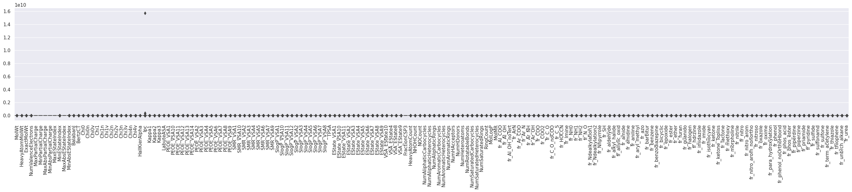
Ipcに非常に大きな外れ値が混ざっているので、これも削除します。
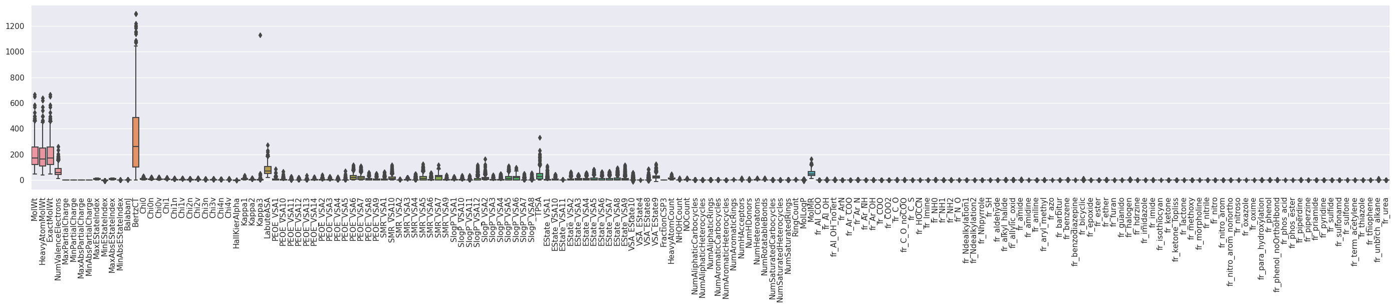
x = x.drop("Ipc", axis=1)
IPC削除前
IPC削除後
今回はコード忘備録も兼ねているので、細かいEDAはすっ飛ばして後々使いまわしたいコードを書きます。
ダブルクロスバリデーションによるPLSモデルの評価
材料開発界隈では、サンプルサイズが小さいことが常なので、train test splitでtrain dataを削る余裕がありません。一方で、全データ学習してハイパーパラメータ調整 (HPO) してクロスバリデーション (CV) をしては、評価用データの情報がHPO時にリークして、評価値を過剰評価してしまいます。ダブルクロスバリデーションでは、CVを入れ子にすることでこの問題に対応しています。train test splitでは、まずデータはtrainとtestにわけて、trainデータのCV評価値を見ながらHPOして、trainデータのみで決定されたモデルでtestデータを評価するといった流れになります。ダブルクロスバリデーションでは、train-test-splitの部分もクロスバリデーションと同様にK分割して、全データをリークさせずに評価用データとして利用するといった方法になります。(詳しくは金子研の解説参照)
以下のコードは、sklearn APIを利用してダブルクロスバリデーションを実装して、以下の項目を確認するものとなります。
- ダブルクロスバリデーション予測値を計算して、yyプロットと評価値を計算
- 各inner cvでfitされたモデルの偏回帰係数を取り出して確認
ダブルクロスバリデーションによるモデルの学習
pipe = make_pipeline(StandardScaler(), VarianceThreshold(), PLSRegression())

inner_cv = KFold(n_splits=5, shuffle=True, random_state=0)
outer_cv = KFold(n_splits=5, shuffle=True, random_state=1)

train_size = 20

params = {"plsregression__n_components": range(1, min(x.shape[1], train_size))}
gscv = GridSearchCV(pipe,
                    params,
                    scoring="neg_mean_absolute_error",
                    cv=inner_cv
                    )

res_dcv = cross_validate(gscv,
                         x,
                         y,
                         scoring=["neg_mean_absolute_error", "neg_root_mean_squared_error"],
                         cv=outer_cv,
                         verbose=1,
                         return_train_score=True,
                         return_estimator=True,
                         )
上記のコードはグリッドサーチCVでHPOしていますが、optunaでsklearn APIに組み込みやすいOptunaSearchCVというクラスを見つけたので、それを使ってみます。以下のコードを使用すると、ベイズ最適化でパラメータサーチができます。
pipe = make_pipeline(VarianceThreshold(), StandardScaler(), PLSRegression())

inner_cv = KFold(n_splits=5, shuffle=True, random_state=0)
outer_cv = KFold(n_splits=5, shuffle=True, random_state=1)

train_size = 20

params = {"plsregression__n_components": IntDistribution(1, min(x.shape[1], train_size))}
opcv = OptunaSearchCV(pipe,
                      params,
                      scoring="neg_mean_absolute_error",
                      cv=inner_cv,
                      verbose=-1
                     )

res_dcv = cross_validate(opcv,
                         x,
                         y,
                         scoring=["neg_mean_absolute_error", "neg_root_mean_squared_error"],
                         cv=outer_cv,
                         verbose=1,
                         return_train_score=True,
                         return_estimator=True,
                         )
学習はこのコードでおしまいです。sklearn様様ですね。
さて、ここから
- ダブルクロスバリデーション予測値と評価値の計算
- 各foldの偏回帰係数
をやっていきます。
ダブルクロスバリデーション予測値の計算
res_dcvにはouter cvの様々の情報が入っていますが、この中のestimatorにinner cvで学習されたモデルの情報が入っています。
def calc_dcv_prediction(inner_gscvs, X, cv):
    fold = np.zeros(X.shape[0], dtype=int)
    dcv_prediction = np.zeros(X.shape[0], dtype=float)
    for i, (inner_gscv, indecies) in enumerate(zip(inner_gscvs, cv.split(X)), 1):
        model = inner_gscv.best_estimator_
        test_index = indecies[1]
        fold[test_index] = i
        dcv_prediction[test_index] = model.predict(X.iloc[test_index, :]).reshape(-1)

    dcv_prediction = pd.DataFrame(np.vstack([fold, dcv_prediction]).T,
                                  index=X.index,
                                  columns=["fold", "predicted"])

    return dcv_prediction

pred_y_dcv = calc_dcv_prediction(res_dcv["estimator"], x, outer_cv)
これで、outer cvのどのfoldで評価されたサンプルであるかとダブルクロスバリデーション予測値が得られます。
実測との相関をyy plotで、予測精度を評価指標で見積もってみましょう。
def yy_plot(observed, predicted):
    g = sns.JointGrid(x=observed, y=predicted)
    g.plot_joint(sns.scatterplot)
    g.plot_marginals(sns.histplot)

    g.ax_joint.set_xlabel("Observed")
    g.ax_joint.set_ylabel("Predicted")

    axis_min = min(*g.ax_joint.set_xlim(), *g.ax_joint.set_ylim())
    axis_max = max(*g.ax_joint.set_xlim(), *g.ax_joint.set_ylim())
    g.ax_joint.set_xlim(axis_min, axis_max)
    g.ax_joint.set_ylim(axis_min, axis_max)
    g.ax_joint.plot([axis_min, axis_max], [axis_min, axis_max], "k--")
    g.ax_joint.set_aspect("equal", adjustable="box")

    return g


def calc_metrics(observed, predicted):
    metrics = {
        "Q2": r2_score(observed, predicted),
        "MAE": mean_absolute_error(observed, predicted),
        "RMSE of OOF": mean_squared_error(observed, predicted, squared=False),
    }
    metrics = pd.DataFrame(metrics, index=["score"])

    return metrics


yy_plot(y, pred_y_dcv["predicted"])
plt.show()
display(calc_metrics(y, pred_y_dcv["predicted"]))
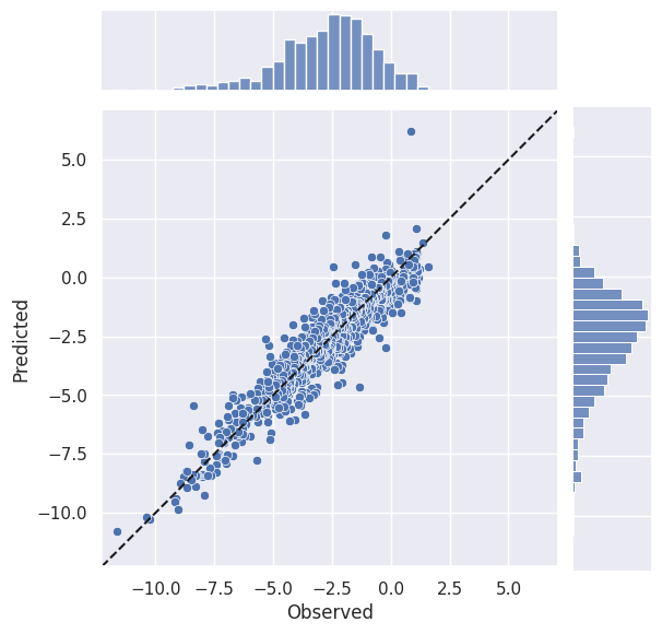
データ数が少ないMI界隈では、CVの評価値として各foldの評価値の平均値では値のばらつきが非常に大きく使い物にならないことがしばしばあります (LeaveOneOutでは$R^2$自体計算不可)。そこで実測値とout of fold predictionを突き合わせて評価指標を計算することが多いです。
実測値とout of fold predictionを突き合わて計算した決定係数は$Q^2$と記載されることが多いです。統計量としての性質はわかりませんが、あまり好ましい性質はないはずだと思っています。一方で、モデルに入力した特徴量と目的変数間の相関の程度を見積もるには便利な指標なので、材料特性に効いている変数を調べたいケースではそれなりに有用だと思っています。(このあたりはエビデンスが薄いです…🙇♂️)
MAEについては、各foldの平均と実測値とout of fold predictionで計算した場合で変わりません。
RMSEは常に「各foldの平均」$\leq$「実測値とout of fold predictionで計算した場合」(詳細) です。より保守的な指標になるので、私はCVの評価指標としてあまり気にせず使っています。
ついでに、入力データと出力データをまとめたdataframeを作成するコードも書いておきます。
def create_output_file(x, y, pred_y, cv=None):
    pred_y = pd.Series(pred_y, index=y.index, name="prediction")
    res_ = pd.concat([y, pred_y, x], axis=1)
    if cv is not None:
        fold = np.zeros_like(y, int)
        for i, indices in enumerate(cv.split(x), 1):
            test_index = indices[1]
            fold[test_index] = i
        fold = pd.Series(fold, index=y.index, name="fold")
        res_ = pd.concat([fold, res_], axis=1)

    return res_


df_out = create_output_file(x, y, pred_y_dcv["predicted"], outer_cv)
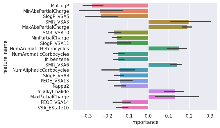
各foldの偏回帰係数
モデルの汎化性能は前章のダブルクロスバリデーション予測値を元にした計算で見積もることができました。汎化性能が良さげなモデルが学習できたとて、そのモデルはどの特徴量を見て汎化誤差を抑えることができているのでしょうか?その答えを偏回帰係数 (決定木ベースの手法の場合は特徴量重要度) で探りに行きます。
今回のコードでは、estimatorに分散0の特徴量削除、標準化の処理、PLS回帰を繋いだpipelineが入っているので、PLSで学習される前に分散0の特徴量が削除され、GridSearchCVに放り込んだXとPLSで学習されるXでは、特徴量が異なる可能性があります。それをケアしながら、偏回帰係数を取り出していき、その平均値と標準偏差を描画します。
def get_coef_of_each_fold(inner_gscvs, X):
    coefs_ = []
    for i, inner_gscv in enumerate(inner_gscvs):
        best_pipe = inner_gscv.best_estimator_
        coef = best_pipe.steps[-1][-1].coef_.reshape(-1)
        best_steps = dict(best_pipe.steps)
        feature_names = best_steps["standardscaler"].feature_names_in_[best_steps["variancethreshold"].get_support()].reshape(-1)
        coef = pd.DataFrame(coef, index=feature_names, columns=[f"fold{i + 1}"])
        coefs_.append(coef)

    coefs_ = pd.concat(coefs_, axis=1, join="outer")

    return coefs_


def plot_cv_feature_importance(cv_feature_importance):
    fold_names = cv_feature_importance.columns
    cv_feature_importance.index.name = "feature_name"
    cv_feature_importance = cv_feature_importance.reset_index()

    display(cv_feature_importance)

    _plotting_data = cv_feature_importance.melt(id_vars=["feature_name"],
                                                value_vars=fold_names,
                                                var_name="fold",
                                                value_name="importance"
                                                ).dropna(axis=0)

    _order = _plotting_data.groupby("feature_name").mean().abs().sort_values("importance", ascending=False).index
    if len(_order) > 20:
        _order = _order[:20]

    sns.barplot(data=_plotting_data,
                x="importance",
                y="feature_name",
                order=_order,
                palette="husl"
                )
    plt.show()


cv_coefs = get_coef_of_each_fold(res_dcv["estimator"], x)
plot_cv_feature_importance(cv_coefs)
何でこんな面倒なことをするの?
MIでは、「材料特性に影響を寄与する因子は何なのか?」を知りたいケースが非常に多いです。機械学習の志向とは真逆ですが、ニーズがあるので私達はそれに答えなければなりません。サンプルサイズが大きければ、train test splitしてtest dataで汎化性能を確認できたら、SHAPなどのXAIでモデルを解釈するという流れが多いかと思います。MIでは、前述の通りtrain test splitをする余裕がなく、CVでモデルの評価をして、全データ学習をし直してモデルの解釈をする場合が多いです。ここで私は、「CVで汎化性能を確認できたモデルはあくまでCVで学習したモデルであって、全データ学習をしたモデルではないはず。それなのにtrainデータの挙動にシビアに影響を受けるスモールデータ解析で汎化性能を確認できていない全データ学習モデルの解釈を元に議論を進めていいのか?」と疑問を持ちました。そこで、今回のように各CVのモデルの挙動をより詳細に確認しようと思ったわけです。
各CVのモデルを元にモデルの解釈をしていけばいいなら、CV各モデルをXAIで解釈すればいいのでは?とも思いましたが、計算量が多い上、出力値が多すぎてどのようにまとめれば解釈をしやすいのかわかりませんでした。そこで私なりの妥協案として考えたものが、「本記事のようにCV各モデルのモデル解釈と、全データ学習し直したモデルの解釈が同じであれば、CVで汎化性能を見積もったモデルと全データ学習したモデルの挙動が大体一致していると判断して、全データ学習モデルをXAIで解釈していく」という手順です。
今回は初めての投稿ということで、適当にPLSでモデルを組みましたが、本来このような取り組みが意味を成すのは、RandomForestやGBDT系のモデルだと思っています (PLSはシンプルなモデルなので、CVと全データ学習モデルの間の乖離が少ないはずなので)。今後、RandomForest, GBDT系版も投稿しようと思います。