はじめに
格子計算プログラム生成言語Formuraを使ってみる。
その2では、一次元熱伝導方程式を解いてみた。今回はそれをそのまま二次元化しよう。
YAMLファイル
YAMLファイルの修正は簡単だ。
一次元系で
gs.yaml
length_per_node: [64.0]
grid_per_node: [64]
と書いていたのを
gs.yaml
length_per_node: [64.0, 64.0]
grid_per_node: [64, 64]
と修正するだけである。
Formuraファイル
まず、次元の宣言を1から2にして、軸にyも追加しよう。
gs.fmr
dimension :: 2
axes :: x,y
次に、isCenterとdiffを二次元化しよう。そのまんまなので難しくないと思う。
gs.fmr
isCenter = fun(i,j,w) (fabs(total_grid_x/2-i) < w) && (fabs(total_grid_y/2-j) < w)

diff = fun(q) (q[i+1,j] + q[i-1,j] + q[i,j+1] + q[i,j-1] - 4.0*q[i,j])
合わせて、初期化関数initを修正する。
gs.fmr
begin function u = init()
  double [] :: u
  u[i,j] = if isCenter(i,j,3) then 0.7 else 0.0
end function
驚くべきことに、時間発展関数は一次元の場合から修正の必要がない。
gs.fmr
begin function u2 = step(u)
  u2 = u + diff(u) * dt
end function
まとめるとこんな感じ。
gs.fmr
dimension :: 2
axes :: x,y

double :: dt = 0.2
double :: Du = 0.05

extern function :: fabs

isCenter = fun(i,j,w) (fabs(total_grid_x/2-i) < w) && (fabs(total_grid_y/2-j) < w)

diff = fun(q) (q[i+1,j] + q[i-1,j] + q[i,j+1] + q[i,j-1] - 4.0*q[i,j])

begin function u = init()
  double [] :: u
  u[i,j] = if isCenter(i,j,3) then 0.7 else 0.0
end function

begin function u2 = step(u)
  u2 = u + diff(u) * dt
end function
main関数
次に、Formuraが吐いたc言語を使う呼び出しファイルの修正である。こちらも、main関数は修正の必要がない。ファイルを吐く関数dumpを二重ループに修正するだけである。
main.cpp
void dump(Formura_Navi &n) {
  char filename[256];
  static int index = 0;
  sprintf(filename, "data/%03d.dat", index);
  index++;
  std::cout << filename << std::endl;
  std::ofstream ofs(filename);
  for (int ix = 0; ix < n.total_grid_x; ix++) {
    for (int iy = 0; iy < n.total_grid_y; iy++) {
      int ix2 = (ix - n.offset_x + n.total_grid_x) % n.total_grid_x;
      int iy2 = (iy - n.offset_y + n.total_grid_y) % n.total_grid_y;
      double v = formura_data.u[ix2][iy2];
      ofs << ix << " ";
      ofs << iy << " ";
      ofs << v << std::endl;
    }
    ofs << std::endl;
  }
}
ここで、オフセットの分場所がずれるので、それをそれぞれ、
      int ix2 = (ix - n.offset_x + n.total_grid_x) % n.total_grid_x;
      int iy2 = (iy - n.offset_y + n.total_grid_y) % n.total_grid_y;
と補正するのは一次元と同様である。
以上をすべてまとめると以下のようになろう。
main.cpp
# include "gs.h"
# include <fstream>
# include <iostream>

void dump(Formura_Navi &n) {
  char filename[256];
  static int index = 0;
  sprintf(filename, "data/%03d.dat", index);
  index++;
  std::cout << filename << std::endl;
  std::ofstream ofs(filename);
  for (int ix = 0; ix < n.total_grid_x; ix++) {
    for (int iy = 0; iy < n.total_grid_y; iy++) {
      int ix2 = (ix - n.offset_x + n.total_grid_x) % n.total_grid_x;
      int iy2 = (iy - n.offset_y + n.total_grid_y) % n.total_grid_y;
      double v = formura_data.u[ix2][iy2];
      ofs << ix << " ";
      ofs << iy << " ";
      ofs << v << std::endl;
    }
    ofs << std::endl;
  }
}

int main(int argc, char **argv) {
  Formura_Navi n;
  Formura_Init(&argc, &argv, &n);
  for (int i = 0; i < 100; i++) {
    Formura_Forward(&n);
    dump(n);
  }
  Formura_Finalize();
}
実行
ファイル生成、コンパイル、実行してみよう。
$ formura gs.fmr
$ g++  main.cpp gs.c
$ rm -rf data
$ mkdir data
$ ./a.out
data/000.dat
data/001.dat
(snip)
data/098.dat
data/099.dat
これをgnuplotに食わせて一気に変換しよう。
set term png
set xra [0:63]
set yra [0:63]
set view map
set size square
unset key

set cbrange[0:0.7]
do for[i=0:99:1]{
  input = sprintf("data/%03d.dat",i)
  output = sprintf("data/%03d.png",i)
  print output
  set out output
  sp input w pm3d
}
実行結果はこんな感じ。
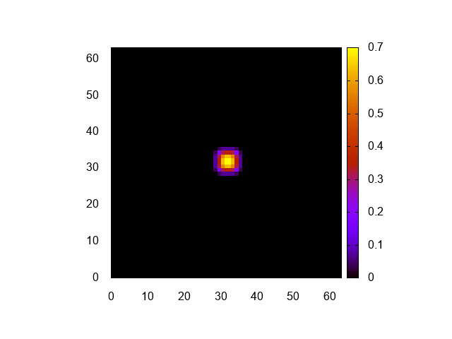


正しく計算できてるみたいですね。
せっかくなのでアニメGIFも置いておきましょうか。

まとめ
一次元熱伝導方程式のファイルを修正して、Formuraに二次元熱伝導方程式を解かせてみた。ファイルを吐くところ以外、ほとんど修正の必要がなく、スムーズにできた。三次元への拡張も簡単であろう。
その4へ続く。