深層学習／ゼロから作るDeep Learning 第７章メモ

1.はじめに

　名著、**「ゼロから作るDeep Learning」**を読んでいます。今回は７章のメモ。
　コードの実行はGithubからコード全体をダウンロードし、ch07の中で jupyter notebook にて行っています。

2.サンプル実装

　テキストで勉強した、Convolution, Pooling を実際に動かしてみるサンプルを実装します。データはMNIST、Convolution のフィルターの重みは学習済みのもの (ch07フォルダーに保存されているparams.pkl) を使います。Convolution, Pooling のコードは、common/layers.py からインポートして使っています。

　まずは、実行してみます。

import sys, os
sys.path.append(os.pardir)  # 親ディレクトリのファイルをインポートするための設定
import numpy as np
import matplotlib.pyplot as plt
from simple_convnet import SimpleConvNet
from common.layers import *  # レイヤーインポート
from dataset.mnist import load_mnist

# 表示関数 (FH, FW) 
def show(filters):    
    FH, FW = filters.shape  
    fig = plt.figure(figsize=(FH*0.1, FW*0.1))  # 表示サイズ指定   
    plt.imshow(((filters)), cmap='gray')
    plt.tick_params(left=False, labelleft=False, bottom=False, labelbottom=False)  # 軸目盛・ラベルを消す
    plt.show()

# MNIST データの読み込み
(x_train, t_train), (x_test, t_test) = load_mnist(flatten=False)
x_train = x_train[5:6]  # 先頭から5番目のデータを選択

# 学習済みパラメータの読み込み
network = SimpleConvNet()  # SimpleConvNet をインスタンス化
network.load_params("params.pkl")  #  パラメータ全体の読み込み 
W1, b1 = network.params['W1'][:1], network.params['b1'][:1]  # 先頭の１つのみにする

# レイヤーの生成
conv = Convolution(W1, b1, stride=1, pad=0)  
pool = Pooling(pool_h=2, pool_w=2, stride=2, pad=0)

# 順伝播
out1 = conv.forward(x_train)  #  畳み込み
out2 = pool.forward(out1)  # プーリング

# 表示
print('input.shape = ',x_train.shape)
show(x_train.reshape(28, 28))
print('filter.shape = ', W1.shape)
show(W1.reshape(5, 5))
print('convolution.shape = ', out1.shape)
show(out1.reshape(24, 24))
print('pooling.shape = ', out2.shape)
show(out2.reshape(12, 12))

　MNIST画像 (1, 1, 28, 28) に、filter55, padding=0, stride=1で畳み込みを行い (1, 1, 24, 24) のデータを、さらにfilter22, padding=0, stride=2でプーリングを行い (1, 1, 12, 12) のデータを得ています。

　それでは、コードのポイントとなる部分を見て行きます。

3.Convolution

# ------------- from common_layers.py -------------
    def forward(self, x):
        FN, C, FH, FW = self.W.shape
        N, C, H, W = x.shape
        out_h = 1 + int((H + 2*self.pad - FH) / self.stride)
        out_w = 1 + int((W + 2*self.pad - FW) / self.stride)

        # ① im2colで画像データを行列データに変換
        col = im2col(x, FH, FW, self.stride, self.pad)

        # ② フィルターをreshapeして2次元配列に展開
        col_W = self.W.reshape(FN, -1).T

        # ③ 行列演算で出力を計算
        out = np.dot(col, col_W) + self.b

        # ④ 出力の形を整える
        out = out.reshape(N, out_h, out_w, -1).transpose(0, 3, 1, 2)

        self.x = x
        self.col = col
        self.col_W = col_W
        return out

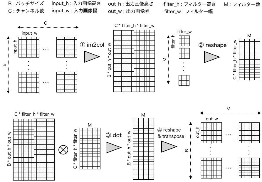
　４次元画像 (バッチサイズ, チャンネル数, 画像高さ, 画像幅) が畳み込み演算によって、どう処理されて行くのかを図で表すとこんな感じ。

　それでは、この中でも特に重要な ① im2col 関数を見てみましょう。

4.im2col

# ------------- from common_layers.py -------------
def im2col(input_data, filter_h, filter_w, stride=1, pad=0):
    N, C, H, W = input_data.shape
    out_h = (H + 2*pad - filter_h)//stride + 1
    out_w = (W + 2*pad - filter_w)//stride + 1
    img = np.pad(input_data, [(0,0), (0,0), (pad, pad), (pad, pad)], 'constant')
    col = np.zeros((N, C, filter_h, filter_w, out_h, out_w))

    # 24*24 フィルターで 5*5 回スライシング (stride=1のとき)
    for y in range(filter_h):  # 5回ループ
        y_max = y + stride*out_h  # y_max = y + 24
        for x in range(filter_w):  # 5回ループ
            x_max = x + stride*out_w  # x_max = x + 24

            # yからy+24まで, xからx+24まで、スライシング
            col[:, :, y, x, :, :] = img[:, :, y:y_max:stride, x:x_max:stride]

    col = col.transpose(0, 4, 5, 1, 2, 3).reshape(N*out_h*out_w, -1)
    return col

　y:y_max:stride, x:x_max:stride は、yからy_maxまでの範囲をstride毎に指定する、xからx_maxまでの範囲をstride毎に指定する、という意味です。

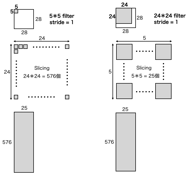
　y_max=y+24, x_max=x+24, stride=1 で、forループはそれぞれ5回の二重ループなので、結局 2424フィルターで55回スライシングすることになります。

　一方で、テキストで勉強した内容から考えると、55フィルターで2424回スライシング となるはずです。それを、コードにするとこんな感じになると思います。

    # 5*5 フィルターで 24*24 回スライシング (stride=1のとき)
    for y in range(0, out_h, stride):    
        for x in range(0, out_w, stride):  
            col[:, :, y, x, :, :] = img[:, :, y:y+filter_h, x:x+filter_w]

　確かに、2424フィルターで55回スライシングも、55フィルターで2424回スライシングも処理する合計の要素数は同じです。結果が同じであるならば、どちらが良いでしょうか？もちろん、前者です。その理由は、処理時間が掛かるforループの回数が圧倒的に少なくて済むからです。

　２つの方法を図で示すと、こんな感じ

5.2つのim2colの比較

　両者の結果が本当に同じなのか確認しておきましょう。オリジナルの im2col と、55フィルターで2424回スライシングする関数 my_im2col を、計算途中のデータを含めてビジュアル化する下記のコードを実行します。

import sys, os
sys.path.append(os.pardir)  # 親ディレクトリのファイルをインポートするための設定
import numpy as np
from dataset.mnist import load_mnist
import matplotlib.pyplot as plt

# データ表示関数 ( x = 表示幅、y = 表示高さ, nx = 列数 )
def show(filters, x, y, nx, margin=1, scale=10):
    FN, C, FH, FW = filters.shape
    ny = int(np.ceil(FN / nx))    
    fig = plt.figure(figsize=(x, y))
    fig.subplots_adjust(left=0, right=1.3, bottom=0, top=1.3, hspace=0.05, wspace=0.05)
    
    for i in range(FN):
        ax = fig.add_subplot(ny, nx, i+1, xticks=[], yticks=[])
        ax.imshow(filters[i, 0], cmap='gray', interpolation='nearest') 
    plt.show()

def my_im2col(input_data, filter_h, filter_w, stride=1, pad=0):
    N, C, H, W = input_data.shape
    out_h = (H + 2*pad - filter_h)//stride + 1  # 出力高さ
    out_w = (W + 2*pad - filter_w)//stride + 1  # 出力幅
    img = np.pad(input_data, [(0,0), (0,0), (pad, pad), (pad, pad)], 'constant')  #　画像パディング  
    col = np.zeros((N, C, out_h, out_w, filter_h, filter_w))  # col計算用行列準備   
    
    # 5*5 フィルターで 24*24 回スライシング (stride=1のとき)
    for y in range(0, out_h, stride):    
        for x in range(0, out_w, stride):  
            col[:, :, y, x, :, :] = img[:, :, y:y+filter_h, x:x+filter_w]
            
    # check1
    print('col.shape after slicing = ', col.shape)
    show(col.reshape(576, 1, 5, 5), x = 3.5, y = 3.5, nx = 24)
    
    # トランスポーズ　＆　リシェイプ
    col = col.transpose(0, 2, 3, 1, 4, 5).reshape(N*out_h*out_w, -1)
    
    # check2
    print('col.shape after transpose & reshape = ', col.shape)
    show(col.reshape(1, 1, 25, 576), x = 18, y =3, nx=1)
    
    return col

def im2col(input_data, filter_h, filter_w, stride=1, pad=0):
    N, C, H, W = input_data.shape
    out_h = (H + 2*pad - filter_h)//stride + 1  # 出力高さ
    out_w = (W + 2*pad - filter_w)//stride + 1  # 出力幅
    img = np.pad(input_data, [(0,0), (0,0), (pad, pad), (pad, pad)], 'constant')  # 画像パディング
    col = np.zeros((N, C, filter_h, filter_w, out_h, out_w))  # col計算用行列準備

    # 24*24 フィルターで 5*5 回スライシング (stride=1のとき)
    for y in range(filter_h):
        y_max = y + stride*out_h
        for x in range(filter_w):
            x_max = x + stride*out_w
            col[:, :, y, x, :, :] = img[:, :, y:y_max:stride, x:x_max:stride]
            
    # check1
    print('col.shape after slicing = ', col.shape)
    show(col.reshape(25, 1, 24, 24), x = 3.5, y = 3.5, nx = 5)
            
    # トランスポーズ　＆　リシェイプ
    col = col.transpose(0, 4, 5, 1, 2, 3).reshape(N*out_h*out_w, -1)
    
    # check2
    print('col.shape after transpose & reshape = ', col.shape)
    show(col.reshape(1, 1, 25, 576), x = 18, y =3, nx=1)
    
    return col

# MNIST データの読み込み
(x_train, t_train), (x_test, t_test) = load_mnist(flatten=False)
x_train = x_train[5:6]  # 先頭から5番目のデータを選択

out1 = my_im2col(x_train, 5, 5)
out2 = im2col(x_train, 5, 5)
print('all elements are same = ', (out1 == out2).all()) # 全ての要素が等しいかどうか  

　前半が my_im2col の結果、後半が im2col の結果です。どちらも col.shape after transpose & reshape は、本当は576行×25列と縦長なのですが、それだと見た目の納まりが悪いので、表示は行と列を入れ替えて25行×576列の横長にしています。そして２つの画像を見ると、確かに同じ模様をしています。

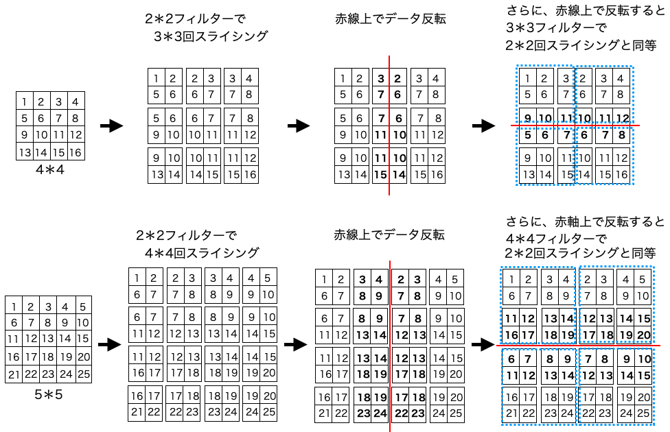
　出力の最終行で、多次元配列の全ての要素を比較した時に True なので、これで my_im2col と im2col は全く同じ結果を出すことが確認できました。一般的には、stride = 1であれば、filter_h * filter_w 回スライシングするだけでOKです。これって凄いテクニックですよね。

　なぜ、こう出来るかについて、直感的に分かる簡単な例を示しておきます。

6.Pooling

# ------------- from common_layers.py -------------
    def forward(self, x):
        N, C, H, W = x.shape
        out_h = int(1 + (H - self.pool_h) / self.stride)
        out_w = int(1 + (W - self.pool_w) / self.stride)

        col = im2col(x, self.pool_h, self.pool_w, self.stride, self.pad)
        col = col.reshape(-1, self.pool_h*self.pool_w)

        arg_max = np.argmax(col, axis=1)
        out = np.max(col, axis=1)
        out = out.reshape(N, out_h, out_w, C).transpose(0, 3, 1, 2)

        self.x = x
        self.arg_max = arg_max
        return out

　４次元画像 (バッチサイズ, チャンネル数, 画像高さ, 画像幅) がPoolingによって、どう処理されて行くのかを図で表すとこんな感じ。

　convolution 同様、pool_h, pool_w, stride, pad を引数に、im2col関数を使って行列を取得し、処理を行っています。