はじめに
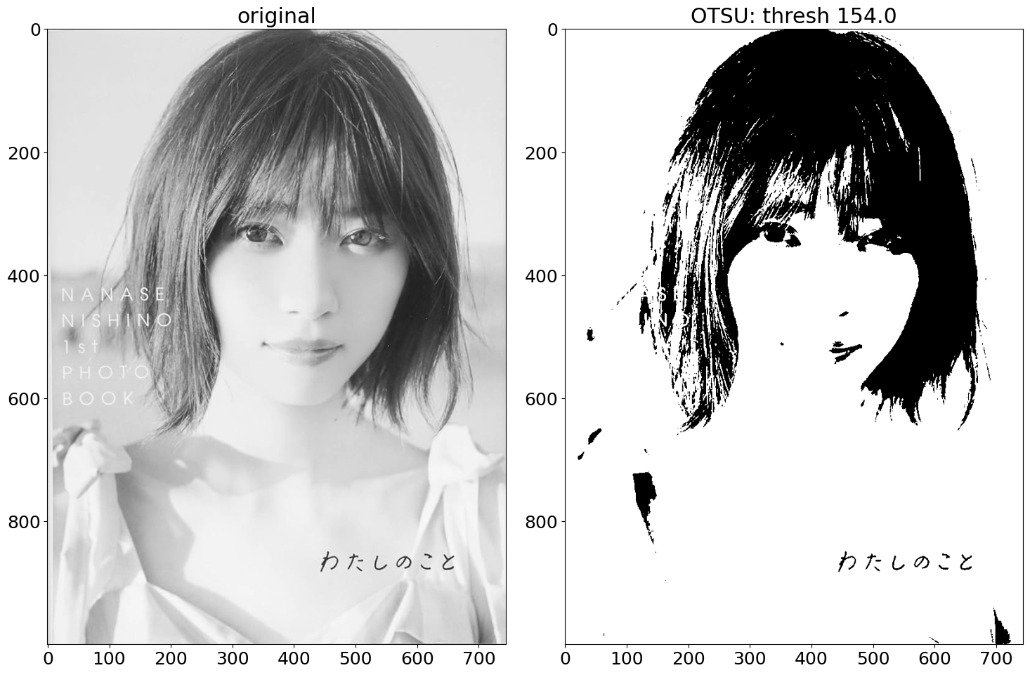
※今回のサンプル画像として、乃木坂46の西野七瀬さんの写真を使用します。元がいい写真なので、今回の処理は蛇足です。

画像の情報量を落として圧縮するための手法の一つに二値化があります。しかし、特定の閾値を基に処理を行う二値化では、画像の構造的な特徴は失われてしまいます。
画像の特徴を維持したまま、二値データとして変換する手法として、疑似濃淡変換(ディザリング)があります。

一例として、組織的ディザリングした画像を拡大すると、二値データで表現されていることがわかります。

今回は自身の理解を深めるために技術記事を書きます。n番煎じです。OpenCVによる画像処理入門 改訂第3版、およびディジタル画像処理 改定新版を参考に実装しました。
ディザリング
概要
ランダムディザリング
ランダムディザリングは画像を走査し、元画像の画素値と $0-255$ の間で生成した乱数を比較し、元画像の画素値が乱数より大きければ $255$ 、小さければ $0$ に二値化する処理を施します。乱数は画素ごとに生成します。今回は画像の高さを $x$ 、幅を $y$、入力の画素値を $I_{src}(x, y)$ 、出力の画素値を $I_{dst}(x, y)$ 、$I_{src}(x, y)$ における乱数を $r(x, y)$ とします。
  I_{dst}(x, y) =
 \begin{cases}
 0 \quad (I_{src}(x, y) < r(x, y))\\
 255  \quad ( otherwise )\\
 \end{cases}

誤差拡散ディザリング
誤差拡散ディザリングは元画像の画素値 $I_{src}(x, y)$ と事前に決めた閾値の値を比較し、元画像の画素値が小さければ $0$、大きければ $255$ に二値化します。上記の処理を行う前に、ひとつ前の画素 $I_{src}(x-1, y)$ の二値化で生じた誤差を $I_{src}(x, y)$ に持ち越して処理を行います。
例として、画素値が以下のようなリストで表される画像かつ閾値が $120$ の時の処理手順を示します。今回、$I_{src}(x, y)$ の処理により生じた誤差を $error(x, y)$ とします。
| y1 | y2 | y3 | y4 | y5 | |
|---|---|---|---|---|---|
| x | 100 | 130 | 10 | 10 | 10 |
- $I_{src}(x, y1)$ が閾値よりも小さいため、$I_{dst}(x, y1)$ を $0$ に二値化
( $I_{src}(x, y1) = 100 < 120 , error(x, y1) = 100$ ) - $I_{src}(x, y2) + error(x, y1)$ が閾値より大きいため、$I_{dst}(x, y2)$ を $255$ に二値化
( $I_{src}(x, y2) + error(x, y1) = 130 + 100 > 120 , error(x, y2) = I_{src}(x, y2) + error(x, y1) - 255 =130 + 100 - 255 = -25 $) - $I_{src}(x, y3) + error(x, y2)$ が閾値より小さいため、$I_{dst}(x, y3)$ を $0$ に二値化
( $I_{src}(x, y3) + error(x, y2) = 10 - 25 < 120 , error(x, y2) = I_{src}(x, y3) + error(x, y2) = 10 - 25 = -15$ ) - 以降繰り返し
説明をシンプルにするため、上述の処理では誤差を右隣の画素に持ち越して計算しています。そのほかに、右、右下、下、左下の画素へ、重みをつけた誤差を拡散させて処理をさせる方法もあります。

組織的ディザリング
組織的ディザリングでは元画像の画素値 $I_{src}(x, y)$ とディザ行列と呼ばれる行列に格納されている閾値 (画素の座標 $(x, y)$ を $4$ で割った剰余のインデックスの値を使用) を比較し、元画像の画素値が小さければ $0$、大きければ $255$ に二値化します。以下にディザ行列の一例であるBeyer 型の行列を示します。
| 0 | 8 | 2 | 10 |
| 12 | 4 | 14 | 6 |
| 3 | 11 | 1 | 9 |
| 15 | 7 | 13 | 5 |

実装
ディザリング手法による違い
# import library
import cv2
import matplotlib.pyplot as plt
import numpy as np

# read image file
path_img = r"" # your img_data_path
img = cv2.imread(path_img)
img_g = cv2.cvtColor(img, cv2.COLOR_BGR2GRAY)
# random dithring
def random_dithering(img):
    img_new = np.zeros(img.size).reshape(img.shape)
    for i in range(img.shape[0]):
        for j in range(img.shape[1]):
            random = np.random.randint(0,255)
            if img[i,j] < random:
                img_new[i,j] = 0
            else:
                img_new[i,j] = 255
    return img_new.astype(np.uint8)

# error-diffusion dithering, 20240814 revise
def error_diffusion_dithering(img, threshold):
    h, w = img.shape
    img_new = np.zeros(img.size).reshape(img.shape)
    error_matrix = np.zeros(img.size).reshape(img.shape)
    for i in range(h):
        for j in range(w):
            value = img[i,j] + error_matrix[i,j]
            if value < threshold:
                img_new[i,j] = 0
                error = value
            else:
                img_new[i,j] = 255
                error = value - 255
            if j + 1 < w:
                error_matrix[i, j + 1] += error * 5 / 16
            if j - 1 >= 0 and i + 1 < h:
                error_matrix[i + 1, j - 1] += error * 3 / 16
            if i + 1 < h:
                error_matrix[i + 1, j] += error * 5 / 16
            if j + 1 < w and i + 1 < h:
                error_matrix[i + 1, j + 1] += error * 3 / 16
    return img_new.astype(np.uint8)

# ordered dithering
def ordered_dithering(img, type = "Bayer"):
    img_new = np.zeros(img.size).reshape(img.shape)
    if type == "Bayer":
        dithe_matrix = np.array([[0, 8, 2, 10],
                             [12, 4, 14, 6],
                             [3, 11, 1, 9],
                             [15, 7, 13, 5]])
    elif type == "Screw":
        dithe_matrix = np.array([[6, 7, 8, 9],
                             [5, 0, 1, 10],
                             [4, 3, 2, 11],
                             [15, 14, 13, 12]])
    elif type == "Screw_skewed":
        dithe_matrix = np.array([[15, 4, 8, 12],
                             [11, 0, 1, 5],
                             [7, 3, 2, 9],
                             [14, 10, 6, 13]])
    elif type == "Mesh":
        dithe_matrix = np.array([[11, 4, 6, 9],
                             [12, 0, 2, 14],
                             [15, 3, 1, 10],
                             [8, 7, 13, 1]])
    elif type == "Intermidiate":
        dithe_matrix = np.array([[12, 4, 8, 14],
                             [11, 0, 2, 6],
                             [10, 3, 1, 9],
                             [15, 5, 7, 13]])
    dithe_matrix *= 16
    for i in range(img.shape[0]):
        for j in range(img.shape[1]):
            if img[i,j] < dithe_matrix[i%4][j%4]:
                img_new[i,j] = 0
            else:
                img_new[i,j] = 255
    return img_new.astype(np.uint8)

# binary by OTSU method
ret, img_otsu = cv2.threshold(img_g, 0, 256, cv2.THRESH_OTSU)
# random dithering
img_random = random_dithering(img_g)
# error_diffusion_dithering
img_error_diffusion = error_diffusion_dithering(img_g, ret)
# ordered_dithering
img_ordered_dithe = ordered_dithering(img_g)

list_img = [img_g, img_otsu, img_random, img_error_diffusion, img_ordered_dithe]
labels = ["original", f"OTSU: thresh {ret}", "random", f"error_diff, thresh {ret}", "ordered_dithe"]


fig, ax = plt.subplots(2,3, tight_layout = True, figsize = (15,15))
ax = ax.flatten()


for i, img in enumerate(list_img):
    ax[i].imshow(img, cmap = "gray")
    ax[i].set_title(labels[i])

plt.show()

見た目の印象では誤差拡散ディザリング、組織的ディザリングがよく画像の特徴を保持していそうです。画像の特徴を基にした元画像との類似性を評価したいため、特徴点マッチング手法の一つである AKAZE を試してみます。以下の参考文献を読んでみると、match オブジェクト内のdistance に特徴点間の距離が格納されているみたいなので、それを取り出してヒストグラムで描画します。
参考文献
- https://qiita.com/komiya_____/items/c024e38959e389442dd0
- https://docs.opencv.org/4.0.0/db/d70/tutorial_akaze_matching.html
## akaze
## create akaze
fig, ax = plt.subplots(2,3, tight_layout = True, figsize = (30,30))
ax = ax.flatten()

fig_h, ax_h = plt.subplots(2,3, tight_layout = True, figsize = (30,30))
ax_h = ax_h.flatten()
for i, img in enumerate(list_img):
   akaze = cv2.AKAZE_create()

   # query
   img_1 = img_g
   img_2 = img
   kp_1, des_1 = akaze.detectAndCompute(img_1, None)
   kp_2, des_2 = akaze.detectAndCompute(img_2, None)

   # create BFMatcher object
   bf = cv2.BFMatcher(cv2.NORM_HAMMING, crossCheck=True)

   # Match descriptors.
   matches = bf.match(des_1,des_2)
   # Sort them in the order of their distance.
   matches = sorted(matches, key = lambda x:x.distance)

   # Draw first 100 matches.
   img_3 = cv2.drawMatches(img_1,kp_1,img_2,kp_2,matches[:100],None,flags=cv2.DrawMatchesFlags_NOT_DRAW_SINGLE_POINTS)

   ax[i].imshow(img_3)
   ax[i].set_title(f"AKAZE_based matching: img_g/{list_sample[i]}")

   # get distance
   distances = []
   for match in matches:
       distances.append(match.distance)
   ax_h[i].hist(distances[:400], bins = 50)
   ax_h[i].set_xlabel("distance")
   ax_h[i].set_ylabel("count")
   ax_h[i].set_title(f"AKAZE_based matching: img_g/{list_sample[i]}")
   print(f"num_match: {list_labels[i]}_{len(matches)}")


見た目の印象と同様に、各ディザリング手法に比して、誤差拡散ディザリングが最も元画像との特徴点間の距離を小さくすることがわかりました。
組織的ディザリングにおけるディザ行列の違い
組織的ディザリングのディザ行列にはBeyer 型のほかに、Screw 型、Screw 変形型、Mesh 型、中間強調型などがあります。これらのディザ行列の違いによるディザリング結果の違いを検討してみます。
- Screw 型
| 6 | 7 | 8 | 9 |
| 5 | 0 | 1 | 10 |
| 4 | 3 | 2 | 11 |
| 15 | 14 | 13 | 12 |
- Screw 変形型
| 15 | 4 | 8 | 12 |
| 11 | 0 | 1 | 5 |
| 7 | 3 | 2 | 9 |
| 14 | 10 | 6 | 13 |
- Mesh 型
| 11 | 4 | 6 | 9 |
| 12 | 0 | 2 | 14 |
| 7 | 8 | 10 | 5 |
| 3 | 15 | 13 | 1 |
- 中間強調型
| 12 | 4 | 8 | 14 |
| 11 | 0 | 2 | 4 |
| 7 | 3 | 1 | 10 |
| 15 | 9 | 5 | 13 |
まず、ディザ行列の違いによる処理結果の違いを強調するため、画像のサイズを落とします。
# resize 33%
dim = (int(img_g.shape[1]/3), int(img_g.shape[0]/3))
img_g_resized = cv2.resize(img_g, dim, interpolation=cv2.INTER_AREA)
fig, ax = plt.subplots(1,2, tight_layout = True)
ax = ax.flatten()
ax[0].imshow(img_g, cmap = "gray")
ax[0].set_title("original")

ax[1].imshow(img_g_resized, cmap = "gray")
ax[1].set_title("resized")

plt.show()

上記画像に対して、ディザ行列を変えて組織的ディザリングを施します。
list_ordered = ["Bayer", "Screw", "Screw_skewed", "Mesh", "Intermidiate"]
fig, ax = plt.subplots(2,3, figsize = (15,15), tight_layout = True)
ax = ax.flatten()
ax[0].imshow(img_g_resized, cmap = "gray")
ax[0].set_title("original")

list_dithe = [img_g_resized]

for i, name in enumerate(list_ordered):
    img_ordered_dithe = ordered_dithering(img_g_resized, type=name)
    ax[i+1].imshow(img_ordered_dithe, cmap = "gray")
    ax[i+1].set_title(f"ordered_dithering: {name}")

    list_dithe.append(img_ordered_dithe)
plt.show()

上述のコードで特徴点マッチングによる類似性を評価すると、Beyer 型がよさそうに見えますが、そこまで大きな差はなさそうな気がします。


おわりに
疑似濃淡変換を理解するために、自身の学びを出力しました。違っている点など見つかれば適宜修正します。ご指摘いただけると感謝です