OpenPoseの概要と実装
1.はじめに
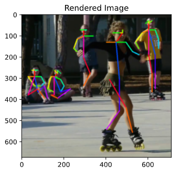
姿勢推定技術で有名なOpenPoseを独自に実装した.本報告では,OpenPoseの理論的な解説,実装時の工夫・苦労した点を書く.図1.に独自実装したOpenPoseの出力結果を示す.大方の姿勢は予測できていることがわかる.しかし,アスペクト比の調整(多段的な推定)を行っていないので,公開されているOpenPoseに比べるとまだ精度は粗く,実用できるレベルではないのが現状である.
 |
|---|
| 図1.独自実装したOpenPoseの出力 |
そもそもOpenPose1とは,リアルタイムに複数人の関節を同時に推定することが出来る姿勢推定アルゴリズムで,姿勢推定アルゴリズムの中で最も有名なアルゴリズムの1つとなっている.実装は論文の著者グループ(カーネギーメロン大学)によって,Githubにオープンソースとして公開されている※.
※ライセンスが独自のものになっており,スポーツの商用利用は不可だったりと厳しいものになっているので注意.
2.OpenPose概要と実装コード抜粋
OpenPoseは,何度かモデルを更新し続けており,論文も複数回提出されている1,2.本報告では,現時点で最新の1についてまとめ,その実装コードを示す.
2.1. モデル構造
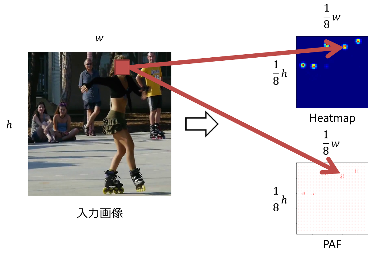
OpenPoseは,図2.のように,キーポイント(関節)らしさを表すHeatmap($\mathrm{S}^t$)とキーポイント同士を結ぶベクトルを表すPart Affinity Field(PAF)($\mathrm{L}^t$)を出力する.HeatmapとPAFのサイズは,それぞれ入力画像に対して$\frac{1}{8}$倍になるように設計されている.(※$\frac{1}{8}$に深い意味はなく,$1$倍だと計算コストが多く,$\frac{1}{8}$より小さいと精度が粗くなってしまうからだと考えられる.)つまり,1x1の領域はそれぞれ,入力画像の8x8に対応するキーポイントらしさ,キーポイント同士の結ぶベクトルを表す.推論の際は,この$\frac{1}{8}$倍とHeatmapとPAFからキーポイント位置を予測することになるので,最低でも4ピクセルの誤差は許容することを暗に示している.
 |
|---|
| 図2.OpenPoseの出力例.サイズは,入力画像に対して1/8倍したものになる.つまり,Heatmap,PAFの1x1の領域はそれぞれ,入力画像の8x8に対応するキーポイントらしさ,キーポイント同士の結ぶベクトルを表す. |
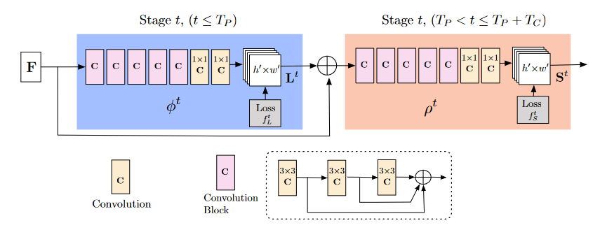
上記を出力するOpenPoseのモデル構造は,以下の図3.のようになる.図中の$\mathrm{F}$は特徴ベクトル抽出層で,VGG193を用いている.桃色のCは点線で囲まれた構造をしており,ResNet4で用いられる残差ブロック(残差を学習する機構)を用いることで,勾配消失を防いでいる(と考えられる).
 |
|---|
| 図3.OpenPoseのモデル構造.図中のFは特徴ベクトル抽出層で,VGG193を用いている.桃色のCはConvolution Blockで点線で囲まれた構造をしている. |
図をよく見ると,PAF$\mathrm{L}^t$を出力する青色のステージ(以下PAFステージ)は,VGGから得られた特徴ベクトル$\mathrm{F}$と,$\mathrm{L}^{t-1}$を入力として,$\mathrm{L}^t$を出力する機構となっている.また,PAFはキーポイント同士の組み合わせ(ボーン)$c$ごとに出力される.数式で表すと以下のようになる.
\begin{align}
\mathrm{L}^t_c &= \phi^t(\mathrm{F}),& t=1 \\
\mathrm{L}^t_c &= \phi^t(\mathrm{F}, \mathrm{L}^{t-1}_c), &otherwize \tag{1}
\end{align}
Heatmap$\mathrm{S}^t$を出力する橙色のステージ(以下Heatmapステージ)は,同様に,VGGから得られた特徴ベクトル$\mathrm{F}$と,PAFステージの最終出力$\mathrm{L}^{T_P}$.$\mathrm{S}^{t-1}$を入力として,$\mathrm{S}^t$を出力する機構となっている.また,Heatmapはキーポイント$j$ごとに出力される.数式で表すと以下のようになる.
\begin{align}
\mathrm{S}^t_j &= \rho^t(\mathrm{F}, \mathrm{L}^{T_P}_j),& t=T_P+1 \\
\mathrm{S}^t_j &= \rho^t(\mathrm{F}, \mathrm{L}^{T_P}_j, \mathrm{S}^{t-1}_j), &otherwize \tag{2}
\end{align}
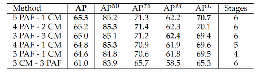
Heatmapステージ,PAFステージのそれぞれの最適数は,表1.に示すように,PAFステージ5個,Heatmapステージ1個であることが報告されている.(私は,PAFステージ4個,Heatmapステージ2個で実装した.)
| 表1.各Heatmapステージ,PAFステージ数ごとの精度比較.PAFステージ5個,Heatmapステージ1個が最も高い精度であることが報告されている. |
|---|
 |
2.2. 学習用Heatmapの生成
概要
Heatmapはキーポイント$j$ごとに作成される.
学習用のHeatmapの作成には,画像内の人物$k$のキーポイント$j$の正解座標$\mathrm{\mathbf{x}}_{j,k}$に対して,以下の2次元のガウス関数を用いる.
\begin{align}
\mathrm{S}^*_{j,k}(\mathrm{\mathbf{p}}) = \exp{\left( -\frac{\lVert \mathrm{\mathbf{p}}-\mathrm{\mathbf{x}}_{j,k} \rVert ^2_2}{\sigma^2} \right)} \tag{3}
\end{align}
ここで,$\mathrm{\mathbf{p}}$は画像内の位置座標を表す.
ガウス関数の性質により,中心から離れれば離れるほど値(キーポイントらしさ)は小さくなる.値が小さくなる度合いを$\sigma$で調節する.
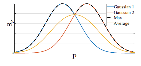
(3)式で得られた人物$k$ごとのHeatmap$\mathrm{S}^*_{j,k}$は$k$に対して最大値を取ることで,最終的な学習用Heatmapを作成している.平均を取らずに最大値を取る理由は,Heatmapが不必要に平滑化されるのを防ぐためである.
\mathrm{S}^*_{j}(\mathrm{\mathbf{p}}) = \max_k \mathrm{S}^*_{j,k}(\mathrm{\mathbf{p}}) \tag{4}
 |
|---|
| 図4.人物ごとにあるHeatmapに対して,最大値を取る理由.平均を取ると,不必要に平滑化されてしまい,対象のキーポイントの座標が移動してしまうことがわかる. |
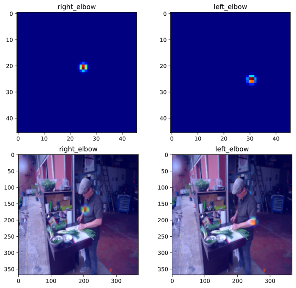
図4.に正解座標$\mathrm{\mathbf{x}}_{j,k}$から作成されたHeatmapを示す.上側が入力画像の$\frac{1}{8}$倍(2.1.参照)の学習に与えるHeatmap$\mathrm{S}^*_j$である.下側は,デバッグ用に実際の入力画像にHeatmapを重畳したものである.
つまり,(2)式の$\mathrm{S}^t_j$は,図4の上側に示されるようなHeatmapを出力することが望まれる.
 |
|---|
| 図5.学習用Heatmapの作成. |
実装コード
コードは以下のように実装した.(3)式とは異なり,上述のリンクにある実装では指数部分を0.5倍していた(ガウス分布を意識した?)ので,本報告もそれらに合わせる.また,$\mathrm{S}^*_j \lt 0.01$は全て0にしている.
また,(3)式の$\mathrm{\mathbf{p}}$はあくまでも入力画像での座標であるため,$\frac{1}{8}$倍サイズのHeatmapとはずれがあることに注意が必要である.そのため,以下の部分で補正している.
※xycoordsは(h,w,2=(x,y))のShapeで,xycoods[y][x][0]=x,xycoods[y][x][1]=yを満たす.
# move coordinates to proper position in original image
# x
stride = orig_size[0] / fmap_size[0]
xycoords[..., 0] = xycoords[..., 0]*stride + stride/2 - 0.5
# y
stride = orig_size[1] / fmap_size[1]
xycoords[..., 1] = xycoords[..., 1]*stride + stride/2 - 0.5
def keypoints2gaussmap_numpy(kpts, vis, orig_size, fmap_size, sigma, method='max', add_background=False):
    """Convert keypoints into heatmap generated by gauusian

    Args:
        kpts (ndarray): The keypoints array, shape = (person_num, keypoint_num, 2=(x,y))
        vis (ndarray): The visibility boolean array, shape = (person_num, keypoint_num)
        orig_size (2d-tuple): (width(int), height(int))
        fmap_size (2d-tuple): (width(int), height(int))
        sigma (float): The standard deviation for gauusian
        method (str, optional): The aggregation method. Defaults to 'max'.
        add_background (bool): Whether to add background confidence map. Default by False

    Raises:
        ValueError: when the given method is invalid
        ValueError: when the given vis is not boolean ndarray

    Returns:
        [ndarray]: The heatmaps, shape = (keypoint_num+1, height, width)
                    Note that the last index of first dimension will represent background's heatmap

    """
    _support_method = ['max', 'average']
    if method not in _support_method:
        raise ValueError('method must be {}, but got {}'.format(_support_method, method))

    if not (isinstance(vis, np.ndarray) and vis.dtype == np.bool):
        raise ValueError('vis must be boolean ndarray')

    # restore keypoints by size
    keypoints = kpts.copy()
    keypoints[..., 0] *= orig_size[0]
    keypoints[..., 1] *= orig_size[1]

    width, height = fmap_size
    # shape = (height, width, 2=(x, y))
    xycoords = generate_coordsmap(width, height)
    # move coordinates to proper position in original image
    # x
    stride = orig_size[0] / fmap_size[0]
    xycoords[..., 0] = xycoords[..., 0]*stride + stride/2 - 0.5
    # y
    stride = orig_size[1] / fmap_size[1]
    xycoords[..., 1] = xycoords[..., 1]*stride + stride/2 - 0.5

    heatmaps = []
    for keypoint_j in range(keypoints.shape[1]):
        hmap = []
        for person_i in range(keypoints.shape[0]):
            if not vis[person_i, keypoint_j]:
                continue
            gaussian = np.exp(-0.5*np.linalg.norm(xycoords - keypoints[person_i, keypoint_j].reshape(1, 1, 2), axis=-1)**2/sigma**2)
            gaussian[gaussian < 0.01] = 0
            hmap += [gaussian.reshape(height, width)]

        if len(hmap) == 0:
            hmap += [np.zeros((height, width))]

        if method == 'max':
            hmap = np.maximum.reduce(np.array(hmap))
        elif method == 'average':
            hmap = np.array(hmap).mean(axis=0)
        else:
            raise ValueError('Bug')
        heatmaps += [hmap]

    # add background heatmap
    if add_background:
        heatmaps += [np.maximum(1-np.max(np.array(heatmaps), axis=0), 0.)]

    return np.array(heatmaps, dtype=np.float32)
入力画像の$\frac{1}{8}$倍のサイズから座標値を作成するgenerate_coordsmapは以下のように実装した.
def generate_coordsmap(width, height):
  """Generate coodinates map from (width, height)

  Args:
      width (int): The width of map
      height (int): The height of map

  Returns:
      [ndarray]: Generated map, shape = (height, width, 2=(x, y))
  """
  # create coordinates array
  """
  >>> x = np.arange(3)
  >>> y = np.arange(2)
  >>> xx, yy = np.meshgrid(x, y)
  >>> xx
  array([[0, 1, 2],
      [0, 1, 2]])
  >>> yy
  array([[0, 0, 0],
      [1, 1, 1]])
  >>> np.concatenate([xx.reshape(-1,1), yy.reshape(-1,1)], axis=-1).reshape(2, 3, 2)
      array([[[0, 0],
              [1, 0],
              [2, 0]],

          [[0, 1],
              [1, 1],
              [2, 1]]])
  """
  # height => x, width => y
  x, y = np.arange(height), np.arange(width)
  # note that meshgrid(x, y) will count up y first.
  # xx => height, yy => width
  xx, yy = np.meshgrid(y, x)
  # shape = (height, width, 2=(x, y))
  xycoords = np.concatenate([xx.reshape(-1,1), yy.reshape(-1,1)], axis=-1).reshape(height, width, 2)

  return xycoords
2.3. 学習用Part Affinity Fieldの生成
概要
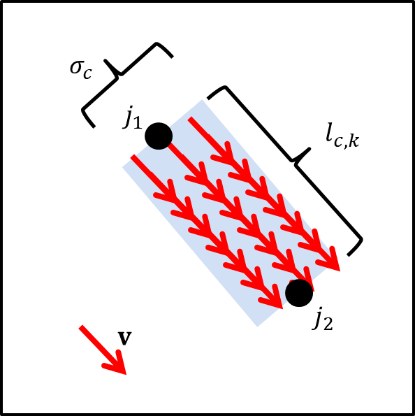
PAFはキーポイントの組み合わせ(ボーン)$c=(j_1, j_2)$($j_1, j_2 \in$キーポイントの集合)ごとに作成される.
学習用のPAFは,画像内の人物$k$のボーン$c$に対して,以下のように作成される.
 |
|---|
| 図6.PAFの作成イメージ図.薄い青色の領域外は全て0ベクトルとなる. |
数式で表すと以下のようになる.
\begin{align}
\mathrm{L}^*_{c,k}(\mathrm{\mathbf{p}}) =
\begin{cases}
 &\mathrm{\mathbf{v}}, & \text{$\mathrm{\mathbf{p}}$がボーン$c$内} \\
 &\mathrm{\mathbf{0}}, & otherwise \tag{5}
\end{cases}
\end{align}
$\mathrm{\mathbf{v}}$は
\mathrm{\mathbf{v}}=\frac{\mathrm{\mathbf{x}}_{j_2,k} - \mathrm{\mathbf{x}}_{j_1,k}}{\lVert \mathrm{\mathbf{x}}_{j_2,k} - \mathrm{\mathbf{x}}_{j_1,k} \rVert _2}
の単位ベクトルである.$\mathrm{\mathbf{p}}$がボーン$c$内にあるかどうかは以下で判断する.
\begin{align}
0 \leq \mathrm{\mathbf{v}} \cdot (\mathrm{\mathbf{p}}-\mathrm{\mathbf{x}}_{j_1,k}) \leq l_{c,k} \text{ and } \lvert \mathrm{\mathbf{v}}_{\bot} \cdot (\mathrm{\mathbf{p}}-\mathrm{\mathbf{x}}_{j_1,k}) \rvert \leq \sigma_{c} \tag{6}
\end{align}
ただし,$l_{c,k}$は以下のように求められる関節間の距離,
l_{c,k}=\lVert \mathrm{\mathbf{x}}_{j_2,k} - \mathrm{\mathbf{x}}_{j_1,k} \rVert _2
$\mathrm{\mathbf{v}}_{\bot}$は$\mathrm{\mathbf{v}}$の垂直単位ベクトル,$\sigma_c$は垂直成分の許容量を表すハイパーパラメータ,である.
(5)式で得られた人物$k$ごとのPAF$\mathrm{L}^*_{c,k}$は$k$に対して,平均(各座標の単位ベクトルの数$n_c(\mathrm{\mathbf{p}})$で除する.)を取ることで,最終的な学習用PAFとしている.
\begin{align}
\mathrm{L}^*_c(\mathrm{\mathbf{p}}) = \frac{1}{n_c(\mathrm{\mathbf{p}})}\sum_k \mathrm{L}^*_{c,k}(\mathrm{\mathbf{p}}) \tag{7}
\end{align}
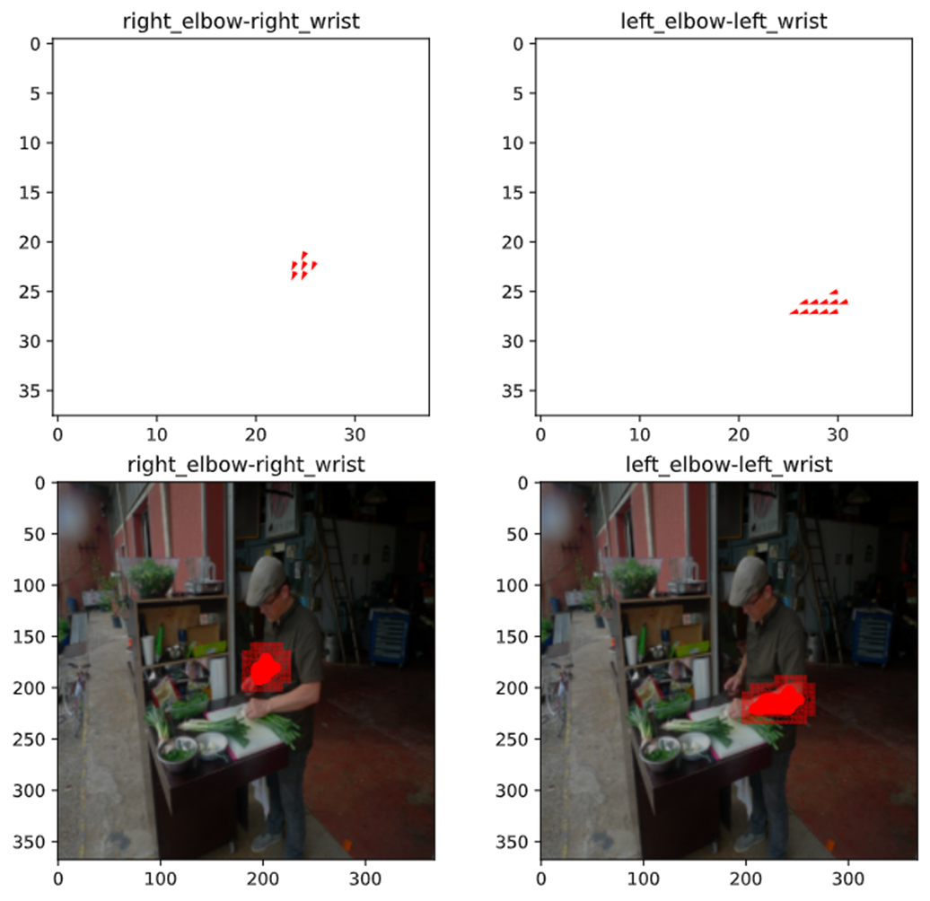
図7.に正解座標$\mathrm{\mathbf{x_{j_1,k}}}$, $\mathrm{\mathbf{x}}_{j_2,k}$から作成されたPAFを示す.上側が入力画像の$\frac{1}{8}$倍(2.1.参照)の学習に与えるPAF:$\mathrm{L}^*_c$である.下側は,デバッグ用に実際の入力画像にPAFを重畳したものである.
つまり,(1)式の$\mathrm{L}^t_c$は,図7の上側に示されるようなPAFを出力することが望まれる.
 |
|---|
| 図7.学習用PAFの生成. |
実装コード
コードは以下のように実装した.特筆すべき点は特にない.
def keypoints2PAF_numpy(kpts, vis, kpt_pairs, orig_size, fmap_size, limb_width):
    """Convert keypoints into PAF

    Args:
        kpts (ndarray): The keypoints array, shape=(person_num, keypoint_num, 2=(x,y))
        vis (ndarray): The visibility boolean array, shape = (person_num, keypoint_num)
        kpt_pairs (list of list): The keypoints pairs
        orig_size (2d-tuple): (width(int), height(int)). Note: not used
        fmap_size (2d-tuple): (width(int), height(int))
        limb_width (float): A limb width.

    Raises:
        ValueError: When the given vis is not boolean ndarray

    Returns:
        ndarray: The PAF array, shape = (pairs_num, height, width, 2=(x, y))
    """
    if not (isinstance(vis, np.ndarray) and vis.dtype == np.bool):
        raise ValueError('vis must be boolean ndarray')

    # restore keypoints by size
    keypoints = kpts.copy()
    keypoints[..., 0] *= fmap_size[0]
    keypoints[..., 1] *= fmap_size[1]

    width, height = fmap_size
    person_num = keypoints.shape[0]
    # shape = (height, width, 2=(x, y))
    xycoords = generate_coordsmap(width, height)

    PAFs = []
    for key_ind1, key_ind2 in kpt_pairs:
        paf = []
        numbers = np.zeros((height, width))
        for person_i in range(keypoints.shape[0]):
            if not vis[person_i, key_ind1] or not vis[person_i, key_ind2]:
                continue
            # calculate the unit vector in the direction of the limb
            # shape = (2=(x,y))
            kpt1, kpt2 = keypoints[person_i, key_ind1], keypoints[person_i, key_ind2]
            dist = np.linalg.norm(kpt2 - kpt1, keepdims=True, axis=-1)
            if dist == 0:
                continue
            dir_u = (kpt2 - kpt1) / np.linalg.norm(kpt2 - kpt1, keepdims=True, axis=-1)


            # calculate perpendicular vectors of the direction unit vector(dir_u)
            dir_perp_u = np.zeros_like(dir_u)
            dir_perp_u[0] = dir_u[1]
            dir_perp_u[1] = -dir_u[0]

            # shape = (height, width, 2=(x,y))
            pos = xycoords.reshape(height, width, 2) - kpt1.reshape(1, 1, 2)

            # scalar
            limb_length = np.linalg.norm(kpt2 - kpt1, axis=-1)

            # boolean indexes. True means it is inside the limb
            # shape = (height, width)
            inner = (dir_u.reshape(1, 1, 2) * pos).sum(axis=-1) # inner product
            limb_bindex = (0 <= inner) & (inner <= limb_length)
            inner = np.abs((dir_perp_u.reshape(1, 1, 2) * pos).sum(axis=-1)) # abs inner product
            limb_bindex = limb_bindex & (inner <= limb_width)

            # shape = (height, width)
            numbers += limb_bindex

            # shape = (height, width, 2)
            limb_bindex = np.broadcast_to(limb_bindex.reshape(height, width, 1), (height, width, 2))

            _paf = np.zeros((height, width, 2))
            np.putmask(_paf, limb_bindex, dir_u.reshape((1, 2)))

            paf += [_paf]

        if len(paf) == 0:
            paf += [np.zeros((height, width, 2))]

        # replace zero into one because of dividint them
        numbers[numbers == 0] = 1

        # shape = (height, width, 2)
        paf = np.array(paf).sum(axis=0)
        paf /= numbers.reshape(height, width, 1)

        PAFs += [paf]

    return np.array(PAFs, dtype=np.float32)
2.4. 学習
概要
2.2.,2.3.に述べたHeatmapとPAFを学習するLoss関数は以下のように,単純な二乗誤差を用い,
\begin{align}
f^t_{\mathrm{L}} &= \sum_c \sum_{\mathrm{\mathbf{p}}} \mathrm{W}(\mathrm{\mathbf{p}}) \cdot \lVert \mathrm{L}_c^t(\mathrm{\mathbf{p}}) - \mathrm{L}_c^*(\mathrm{\mathbf{p}}) \rVert_2^2 \\
f^t_{\mathrm{S}} &= \sum_j \sum_{\mathrm{\mathbf{p}}} \mathrm{W}(\mathrm{\mathbf{p}}) \cdot \lVert \mathrm{S}_j^t(\mathrm{\mathbf{p}}) - \mathrm{S}_j^*(\mathrm{\mathbf{p}}) \rVert_2^2 \tag{8}
\end{align}
各ステージごとの誤差を加算したものを用いる.$\mathrm{W}(\mathrm{\mathbf{p}})$はデータセットの欠損(人物領域が小さすぎる・オクルージョン・キーポイント数が少ない等)を除外する2値マスクである.
$$
f = \sum_{t=1}^{T_P} f^t_{\mathrm{L}} + \sum_{t=T_P+1}^{T_P+T_C} f^t_{\mathrm{S}} \tag{9}
$$
このように中間のステージを同時に学習することで,勾配消失を防いでいる.
実装コード
人物領域が$32\times 32$未満,キーポイントの数が5未満である場合は欠損とみなすようにする.そのため,上記を満たす領域は$\mathrm{W}(\mathrm{\mathbf{p}})=0$でマスクする.コードは以下のようになる.
$32\times 32$未満の人物領域を欠損とみなす理由は,予測されるHeatmapとPAFが入力画像の$\frac{1}{8}$倍であるため,$32\times 32$未満の人物領域はHeatmapやPAF上では$4\times 4$未満の領域になる.人物のキーポイントをすべて表現するにはあまりにも小さいので,これらは欠損値とみなす.
def generate_mask(jsonpath):
    # original code: https://github.com/ZheC/Realtime_Multi-Person_Pose_Estimation/blob/master/training/genCOCOMask.m
    co = _coco.COCO(jsonpath)

    # eg. train2014, val2014
    focus = os.path.splitext(jsonpath)[0].split('_')[-1]

    mask_all_dir = os.path.join(os.path.dirname(jsonpath), 'mask_all', focus)
    os.makedirs(mask_all_dir, exist_ok=True)
    mask_miss_dir = os.path.join(os.path.dirname(jsonpath), 'mask_miss', focus)
    os.makedirs(mask_miss_dir, exist_ok=True)

    # list of dict:=> area, iscrowd, num_keypoints, segmentation, keypoints, image_id, bbox, category_id, id
    all_annotations = co.loadAnns(co.getAnnIds())

    # gather annotations into one image's annotations
    # dict of list of dict, coco_kpt[image_num][person_num][annotation's key]
    annotations_per_img = {}

    for anno in all_annotations:
        curr_id = anno['image_id']
        # for debug
        #if curr_id not in [257, 357]:
        #    continue
        if curr_id not in annotations_per_img.keys():
            annotations_per_img[curr_id] = []

        annotations_per_img[curr_id] += [anno]

    for img_id, annotations in tqdm(annotations_per_img.items()):
        # dict => license, file_name, coco_url, height, width, data_captured, flickr_url, id
        imginfo = co.loadImgs(img_id)[0]

        # create mask
        segmentation_all = np.zeros((imginfo['height'], imginfo['width']), dtype=bool)
        mask_miss = np.zeros_like(segmentation_all, dtype=bool)
        mask_crowd = np.zeros_like(segmentation_all, dtype=bool)

        try:
            for anno in annotations:
                # anno dict:=> area, iscrowd, num_keypoints, segmentation, keypoints, image_id, bbox, category_id, id

                # check this person is annotated
                # seg: list
                seg = anno['segmentation'][0]

                img = Image.new('L', (imginfo['width'], imginfo['height']), 0)
                ImageDraw.Draw(img).polygon(np.array(seg, dtype=int).tolist(), outline=1, fill=1)
                mask = np.array(img, dtype=bool)
                #cv2.imwrite(os.path.join(mask_dir, 'mask_all_test.png'), mask.astype(np.uint8)*255)
                segmentation_all = np.logical_or(mask, segmentation_all)

                # mask for missing
                #if anno['num_keypoints'] <= 0:
                if anno['num_keypoints'] < 5 or anno['area'] < 32*32:
                    mask_miss = np.logical_or(mask, mask_miss)
            mask_miss = np.logical_not(mask_miss)

        except KeyError:
            mask_noanno = co.annToMask(anno).astype(bool)
            mask_crowd = np.logical_xor(mask_noanno,  np.logical_and(segmentation_all, mask_noanno))
            mask_miss = np.logical_not(np.logical_or(mask_miss, mask_crowd))
            #anno['mask_crowd'] = _mask.encode(mask_crowd)

        mask_all = np.logical_or(segmentation_all, mask_crowd)

        # save as image
        filename, _ = os.path.splitext(imginfo['file_name'])
        cv2.imwrite(os.path.join(mask_all_dir, filename + '.png'), mask_all.astype(np.uint8)*255)
        cv2.imwrite(os.path.join(mask_miss_dir, filename + '.png'), mask_miss.astype(np.uint8)*255)
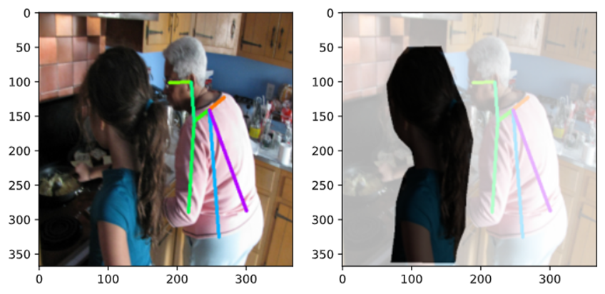
上記により生成されたマスクは以下の図8.のようになる.手前の女性はアノテーションがされていないため,学習の妨げとなり得る.そのため,右図のように,全体を$\mathrm{W}(\mathrm{\mathbf{p}})=0$でマスクしている.
 |
|---|
| 図8.マスク.手前の女性はアノテーションされていない.そのため,その領域は全てマスクする必要がある. |
誤差関数は以下のように実装した.
class OpenPoseLoss(nn.Module):
    def __init__(self, alpha=1, det_loss=None, conf_loss=None, reduction='sum', hnm_ratio=None, rnm_ratio=None):
        """OpenPose Loss function

        Args:
            alpha (float, optional): The coefficient for detection loss and confidence loss. Defaults to 1.
                                     total_loss = det_loss + alpha*conf_loss
            det_loss (nn.Module, optional): The detection loss function. Defaults to None.
                                            If None, set the DetectionLoss module.
            conf_loss (nn.Module, optional): The confidence loss function. Defaults to None.
                                             If None, set the ConfidenceLoss module.
            reduction (str, optional): The reduction method for gathering loss. Defaults to 'sum'
                                       Methods are ['none', 'sum', 'mean']
            hnm_ratio (int, optional): The online negative mining ratio. Default to None
            rnm_ratio (int, optional): The online "RANDOM" negative mining ratio. Default to None
        """
        super().__init__()
        self.alpha = alpha
        self.reduction = reduction
        self.hnm_ratio = hnm_ratio
        self.rnm_ratio = rnm_ratio
        self.gen_mask = gen_mask

        self.det_loss = DetectionLoss(reduction=reduction, hnm_ratio=hnm_ratio, rnm_ratio=rnm_ratio) if det_loss is None else det_loss
        self.conf_loss = ConfidenceLoss(reduction=reduction, hnm_ratio=hnm_ratio, rnm_ratio=rnm_ratio) if conf_loss is None else conf_loss

    def forward(self, masks, predicts, targets):
        """Calculate a loss

        Args:
            masks:
                Tensor: The mask tensor, shape = (b, h, w)
            predicts:
                    list of Tensor: The predicted PAF map tensor for each stage, shape = (b, pairs_num, h, w, 2)
                    list of Tensor: The predicted confidence map tensor for each stage, shape = (b, keypoints_num, h, w)
            targets:
                Tensor: The annotated PAF map tensor, shape = (b, pairs_num, h, w, 2)
                Tensor: The annotated confidence map tensor, shape = (b, keypoints_num, h, w)

        Returns:
            Tensor: A detection loss
            Tensor: A confidence loss
        """
        masks = masks.bool()
        pred_pafs, pred_confs = predicts
        target_pafs, target_confs = targets

        det_loss = self.det_loss(masks, pred_pafs, target_pafs)
        conf_loss = self.conf_loss(masks, pred_confs, target_confs)

        return det_loss, conf_loss

class DetectionLoss(nn.Module):
    def __init__(self, hnm_ratio=None, rnm_ratio=None, reduction='sum'):
        """OpenPose Detection Loss function

        Args:
            reduction (str, optional): The reduction method for gathering loss. Defaults to 'sum'
                                       Methods are ['none', 'sum', 'mean']
            hnm_ratio (int, optional): The online negative mining ratio. Default to None
            rnm_ratio (int, optional): The online "RANDOM" negative mining ratio. Default to None
        """
        super().__init__()
        self.hnm_ratio = hnm_ratio
        self.rnm_ratio = rnm_ratio
        self.reduction = reduction

    def forward(self, masks, predicts, target):
        """Calculate a detection loss

        Args:
            masks: Tensor: The mask tensor, shape = (b, h, w)
            predicts (list of Tensor): The predicted PAF map tensor for each stage, shape = (b, pairs_num, h, w, 2)
            target (Tensor): The annotated PAF map tensor, shape = (b, pairs_num, h, w, 2)

        Returns:
            Tensor: A detection loss
        """
        b, pairs_num, h, w, _ = target.shape
        masks = torch.broadcast_to(masks.unsqueeze(1).unsqueeze(-1), (b, pairs_num, h, w, 2))

        if self.hnm_ratio:
            # shape = (b, pairs_num, h, w)
            posmask = torch.linalg.norm(target, dim=-1) > 1e-6

            posnum = posmask.sum().item()

            hard_sample_nums = int(posnum * self.hnm_ratio)
            random_sample_nums = int(posnum * self.rnm_ratio) if self.rnm_ratio else None
            hard_mask, random_mask = ohem_mask(torch.linalg.norm(predicts, dim=-1), posmask, hard_sample_nums, random_sample_nums)

            masks = posmask | hard_mask | random_mask

            masks = torch.broadcast_to(masks.unsqueeze(-1), (b, pairs_num, h, w, 2))

        if self.reduction in ['sum', 'none']:
            det_losses = [F.mse_loss(predict[masks], target[masks], reduction=self.reduction)/b for predict in predicts]
        else:
            # mean
            det_losses = [F.mse_loss(predict[masks], target[masks], reduction=self.reduction) for predict in predicts]
        #det_losses = [F.mse_loss(predict*masks, target*masks, reduction=self.reduction) for predict in predicts]
        return torch.stack(det_losses).sum()

class ConfidenceLoss(nn.Module):
    def __init__(self, hnm_ratio=None, rnm_ratio=None, reduction='sum'):
        """OpenPose Confidence Loss function

        Args:
            reduction (str, optional): The reduction method for gathering loss. Defaults to 'sum'
                                       Methods are ['none', 'sum', 'mean']
            hnm_ratio (int, optional): The online negative mining ratio. Default to None
            rnm_ratio (int, optional): The online "RANDOM" negative mining ratio. Default to None
        """
        super().__init__()
        self.hnm_ratio = hnm_ratio
        self.rnm_ratio = rnm_ratio
        self.reduction = reduction

    def forward(self, masks, predicts, target):
        """Calculate a confidence loss

        Args:
            masks: Tensor: The mask tensor, shape = (b, h, w)
            predicts (list of Tensor):  list of Tensor: The predicted confidence map tensor for each stage, shape = (b, keypoints_num, h, w)
            target (Tensor): The annotated confidence map tensor, shape = (b, keypoints_num, h, w)

        Returns:
            Tensor: A confidence loss
        """
        b = target.shape[0]
        masks = torch.broadcast_to(masks.unsqueeze(1), target.shape)

        if self.hnm_ratio:
            posmask = target > 1e-6
            posnum = posmask.sum().item()

            hard_sample_nums = int(posnum * self.hnm_ratio)
            random_sample_nums = int(posnum * self.rnm_ratio) if self.rnm_ratio else None
            hard_mask, random_mask = ohem_mask(predicts, posmask, hard_sample_nums, random_sample_nums)

            masks = posmask | hard_mask | random_mask

        if self.reduction in ['sum', 'none']:
            det_losses = [F.mse_loss(predict[masks], target[masks], reduction=self.reduction)/b for predict in predicts]
        else:
            det_losses = [F.mse_loss(predict[masks], target[masks], reduction=self.reduction) for predict in predicts]
        #det_losses = [F.mse_loss(predict*masks, target*masks, reduction=self.reduction) for predict in predicts]
        return torch.stack(det_losses).sum()
Heatmapの誤差関数の注意点
※以下は,あくまで仮説で未検証なので,詳細をご存知の方はご指摘いただきたい.
ここで注意したいのが,mse_lossのreduction引数である.reductionはsum,mean,noneの3種類がある.(8)式に従うならば,当然ながらreduction='sum'(またはnoneを指定した後に.sum())とすべきである.しかしながら,当初はreduction='mean'としていた.違いは,Heatmapのサイズを$(w', h')$とした場合,(8)式を$w' \times h'$で除しているかどうかだけであるが,学習結果は大きく異なる.
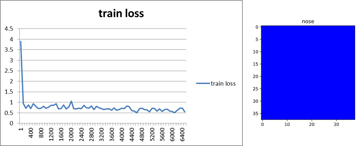
図9に示すように,reduction='mean'の場合,学習曲線はIterationごとに徐々に下がる一方(図だとわかりづらいが明らかに下がっていった)で,そのHeatmapの出力はほぼ全てが0になった.これは,学習率が原論文と同じ(正確には,原論文には記載がなかったため,公式実装のprototxtを参考にした.)ままでreduction='mean'とすると,Lossを平均することで扱う桁数が小さくなり,実質的に勾配が消失したことが原因だと考えられる.実際,学習時のHeatmapのサイズは$38\times 38$であるために,桁数は3桁ほど小さくなる.
 |
|---|
図9.reduction=mean時の学習曲線とHeatmap出力. |
【理論とイメージ】CNNの誤差逆伝播とDeconvolutionまとめのCNNの逆伝搬の数式を用いると,$\frac { \partial J _ { i } } { \partial a _ { m - p , n - q , k ^ { \prime } } ^ { l + 1 } }$が$\frac{1}{38\times 38} \approx 10^{-3}$倍されることがわかる.また,学習用Heatmapは$0\leq \mathrm{S}^*_j(\mathrm{\mathbf{p}}) \leq 1$で,そのほとんどが0である.それ故,先に大部分の0を学習した状態で,局所解から抜け出せなくなったのだと考えられる.
$
\delta _ { m , n , k } ^ { l } = \frac { \partial J _ { i } } { \partial a _ { m , n , k } ^ { l } } = \sum _ { p , q , k ^ { \prime } } \frac { \partial J _ { i } } { \partial a _ { m - p , n - q , k ^ { \prime } } ^ { l + 1 } } \frac { \partial a _ { m - p , n - q , k ^ { \prime } } ^ { l + 1 } } { \partial a _ { m , n , k } ^ { l } }
$$\frac { \partial a _ { m - p , n - q , k ^ { \prime } } ^ { l + 1 } } { \partial a _ { m , n , k } ^ { l } }$の計算は、順伝播の時の計算を参照すると、以下のようになります。
$
\frac { \partial a _ { m - p , n - q , k ^ { \prime } } ^ { l + 1 } } { \partial a _ { m , n , k } ^ { l } } = w _ { p , q , k , k ^ { \prime } } ^ { l + 1 } h ^ { \prime } \left( a _ { m , n , k } ^ { l } \right)
$さらに、$\frac { \partial J _ { i } } { \partial a _ { m - p , n - q , k ^ { \prime } } ^ { l + 1 } }=\delta _ { m - p , n - q , k ^ { \prime } } ^ { l + 1 }$となることに注意すると、最終的に以下のようになります。
$
\delta _ { m , n , k } ^ { l } = h ^ { \prime } ( a _ { m , n , k } ^ { l } )\sum _ { p , q , k ^ { \prime } } \delta _ { m - p , n - q , k ^ { \prime } } ^ { l + 1 } \cdot w _ { p , q , k , k ^ { \prime } } ^ { l + 1 }
$
2.5. 関節領域抽出(NMS)
概要
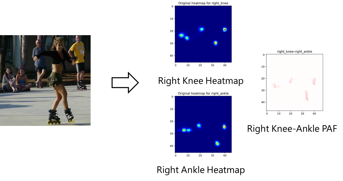
学習が正しく行えると,以下のようにHeatmap,PAFが得られる.
得られたHeatmap,PAFからキーポイント位置・その接続(ボーン)を推定し,骨格情報を構成していく.
 |
|---|
| 図10.HeatmapとPAFの出力結果.図は右膝と右足首のHeatmap及びそれらを繋ぐベクトルを表すPAF. |
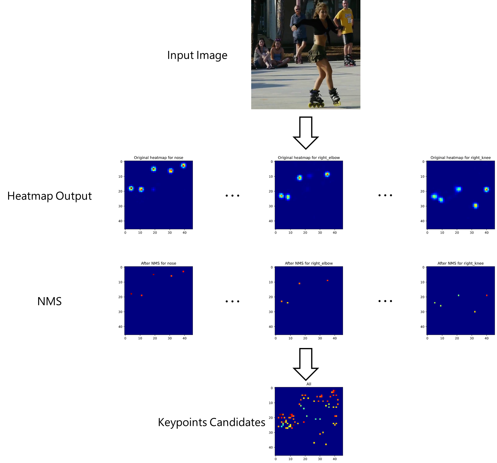
Heatmapは,各ピクセルの領域のキーポイントらしさを表すので,近傍のピクセルは同じキーポイントを表していると考えられる.したがって,近傍のピクセルを1つにまとめる必要がある.そこで,有効なのがNMS(Non-maximum Suppression)である.その名の通り,近傍のピクセルで最大でないものは除く処理である.NMSを適用すると図11.のように近傍のHeatmapが除かれ,1ピクセルにまとまっていることがわかる.
(逆に言えば,Heatmap手法は冗長な予測をしていると考えることもできる.)
 |
|---|
| 図11.NMS適用結果. |
実装コード
実装は簡単で,scipyのmaximum_filterを用いれば良い.
def nms(conf_map):
    """Non-maximum suppression for confidence map

    Args:
        conf_map (ndarray): The confidence map, shape = (b, keypoint_num, h, w)

    Returns:
        ndarray: The confidence map suppressed non-maximum values
    """
    footprint = np.array([[False, True, False],
                            [True, True, True],
                            [False, True, False]])
    footprint = footprint.reshape((1, 1, 3, 3))
    return conf_map*(conf_map == maximum_filter(conf_map, footprint=footprint))
2.6. (2部グラフ)マッチング
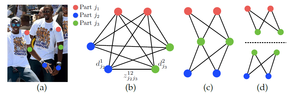
キーポイント位置が推定できたら,次にキーポイント同士を接続する必要がある.この問題は,割り当て問題と考えることができる.ここで,単純に全組み合わせについて,割り当て問題を解こうとすると,図12.(b)のようになる.人体のようにキーポイント同士の組み合わせ(ボーン)が定義されている場合,組み合わせの数は少し削減でき,(c)のようになる.しかし,この(c)の割り当て問題は,NP-Hardな問題である.そこで,OpenPoseでは(d)のように,隣接するキーポイント同士のみの割り当て問題,2部グラフのマッチング問題を考えるという大胆な緩和を行う.このように緩和しても,実験的に問題ないことが示されている.著者はこの理由を,PAFを出力するまでの複数の畳み込み演算により,十分に受容野が大きくなるため,PAFが大域的なContext(前後関係)を学習しているからだと主張している.
 |
|---|
| 図12.キーポイントのマッチング問題. |
(d)のような2部グラフのマッチング問題は,そのボーン(エッジ)のスコアが定義できれば,解くことが可能である.OpenPoseでは,図13.のようにPAFのベクトルをキーポイント候補上で線績分したものをスコアとする.具体的には,
E = \int_u \mathrm{\mathbf{L}}_c(\mathrm{\mathbf{p}}(u)) \cdot \frac{\mathrm{\mathbf{d}}_{j_2} - \mathrm{\mathbf{d}}_{j_2}}{\lVert \mathrm{\mathbf{d}}_{j_2} - \mathrm{\mathbf{d}}_{j_2} \rVert_2} du \tag{10}
とする.このスコアを考えられるボーンごとに(ある右膝に対して,検知された右足首の候補を繋ぐ全てのボーン)計算し,ハンガリアンアルゴリズムで2部グラフのマッチング問題を解けば,最適な隣接するボーンの組み合わせ(図12.(d)の最適解)が得られる.
実装コード
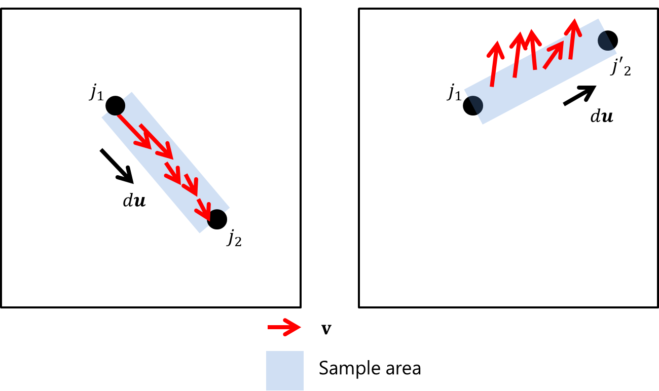
(10)式において,$u$は離散値であるため,実装では,
E \approx \frac{1}{N} \sum_{\mathrm{\mathbf{p}} \in B_{j_1, j_2}^N} \mathrm{\mathbf{L}}_c(\mathrm{\mathbf{p}}) \cdot \frac{\mathrm{\mathbf{d}}_{j_2} - \mathrm{\mathbf{d}}_{j_1}}{\lVert \mathrm{\mathbf{d}}_{j_2} - \mathrm{\mathbf{d}}_{j_1} \rVert_2} \tag{11}
とした.$B_{j_1, j_2}^N$はキーポイント同士のベクトル間
(\mathrm{\mathbf{d}}_{j_2} - \mathrm{\mathbf{d}}_{j_1})
の$N$個の座標値の集合である.なお,$N=10$とした.この線績分の近似は以下の図のようになる.ボーンの方向に寄与するPAFの成分が多ければ多いほど,線積分の値は大きくなる.(左図の${j_1,j_2}$の組み合わせの方が,値が大きくなる.)
 |
|---|
| 図13.線積分の近似イメージ. |
さらに,長さの制約を追加するために,ひと工夫をしている.(この辺りは微妙なので,要改善.)
integrals[i1, i2] = integral_scores.mean() + min(0.5*h/normVec[i1, i2] - 1, 0)
def matching(paf, candInd_with_score, kpt_pairs, sample_nums):
    """Matching proper keypoint pairs from PAF

    Parameters
    ----------
    paf : ndarray
        PAF. shape = (pairs_num, h, w, 2=(x,y))
    candInd_with_score : list of dict
        Candidate Indices with score's list. Dict's keys are;
        'xinds': ndarray, shape = (cand_nums,)
        'yinds': ndarray, shape = (cand_nums,)
        'confs': ndarray, shape = (cand_nums,)
    kpt_pairs : list of list(2d)
        The keypoint pairs list
    sample_nums : int
        A samplimg number on line-integral

    Returns
    -------
    dict
        The matched connections dict. Dict keys are;
        'kpt1s': int ndarray, shape = (size, 2=(x,y))
        'kpt2s': int ndarray, shape = (size, 2=(x,y))
        'conf1s': ndarray, shape = (size,)
        'conf2s': ndarray, shape = (size,)
        'kpairinds': int ndarray, shape = (size,)
        'scores': int ndarray, shape = (size,)
    """
    h, w = paf.shape[:2]

    connections = {"kpt1s": np.empty((0, 2), dtype=int), "kpt2s": np.empty((0, 2), dtype=int),
                   "conf1s": np.empty(0, dtype=np.float32), "conf2s": np.empty(0, dtype=np.float32), "kpairinds": np.empty(0, dtype=int), "scores": np.empty(0, dtype=np.float32)}

    for kpairind, (key1, key2) in enumerate(kpt_pairs):
        ####### line integral ######
        vals1, vals2 = candInd_with_score[key1], candInd_with_score[key2]
        # shape = (h, w)
        pafX, pafY = paf[kpairind, ..., 0], paf[kpairind, ..., 1]
        # shape = (cand_nums1,)
        x1s, y1s, conf1s = vals1['xinds'], vals1['yinds'], vals1['confs']
        # shape = (cand_nums2,)
        x2s, y2s, conf2s = vals2['xinds'], vals2['yinds'], vals2['confs']

        # shape = (cand_nums1, cand_nums2)
        deltaX = np.add.outer(-x1s, x2s)
        deltaY = np.add.outer(-y1s, y2s)
        # 1e-6 means to avoid RuntimeWarining
        normVec = np.sqrt(deltaX**2 + deltaY**2) + 1e-6
        vx, vy = deltaX/normVec, deltaY/normVec

        integrals = np.ones_like(deltaX, dtype=np.float32) * -9999
        for i1 in range(deltaX.shape[0]):
            for i2 in range(deltaX.shape[1]):
                # sample
                # shape = (sample_nums,)
                xinds_sampled = np.linspace(x1s[i1], x2s[i2], sample_nums).astype(np.int8)
                yinds_sampled = np.linspace(y1s[i1], y2s[i2], sample_nums).astype(np.int8)

                # shape = (sample_nums,)
                pafX_sampled = pafX[yinds_sampled, xinds_sampled]
                pafY_sampled = pafY[yinds_sampled, xinds_sampled]

                # integral
                # shape = (sample_nums,)
                integral_scores = (pafX_sampled*vx[i1, i2] + pafY_sampled*vy[i1, i2])

                integrals[i1, i2] = integral_scores.mean() + min(0.5*h/normVec[i1, i2] - 1, 0)
                """
                # condition1: whether each point's paf score at least 80% is greater than threshold
                # condition2: each point's average paf score, penalized for limb length, is greater than a half of height
                if (np.count_nonzero(integral_scores > matching_thres) > 0.8*integral_scores.size) and \
                   (integral_scores.mean() + min(0.5*h/normVec[i1, i2] - 1, 0) > 0):
                    # do integral
                    integrals[i1, i2] = integral_scores.mean() + min(0.5*h/normVec[i1, i2] - 1, 0)
                """

        # assignment by Hungarian algorithm
        # -integrals means "cost" matrix, not score matrix
        m1inds, m2inds = linear_sum_assignment(-integrals)
        m1inds_new, m2inds_new = [], []
        for m1i, m2i in zip(m1inds, m2inds):
            if integrals[m1i, m2i] <= 0:
                continue
            m1inds_new += [m1i]
            m2inds_new += [m2i]

        # shape = (*, 2)
        new_kpt1 = np.concatenate([x1s[m1inds_new].reshape((-1, 1)), y1s[m1inds_new].reshape((-1, 1))], axis=-1)
        connections["kpt1s"] = np.concatenate([connections["kpt1s"], new_kpt1], axis=0)
        new_kpt2 = np.concatenate([x2s[m2inds_new].reshape((-1, 1)), y2s[m2inds_new].reshape((-1, 1))], axis=-1)
        connections["kpt2s"] = np.concatenate([connections["kpt2s"], new_kpt2], axis=0)
        connections["conf1s"] = np.append(connections["conf1s"], conf1s[m1inds_new])
        connections["conf2s"] = np.append(connections["conf2s"], conf2s[m2inds_new])
        connections["kpairinds"] = np.append(connections["kpairinds"], np.array([kpairind]*len(m1inds_new), dtype=int))
        connections["scores"] = np.append(connections["scores"], integrals[m1inds_new, m2inds_new])

        # assignement
        # sort with descending order and got 2d-indices by unravel_index
        # xi, yi = np.unravel_index(np.argsort(integrals, axis=None)[::-1], integrals.shape)

    return connections
この時点でのボーン候補をプロットすると以下のようになる.
 |
|---|
| 図14.2部グラフマッチング問題を解いた後のプロット図. |
2.7. ボーンから人物構築
最後に,2.6.で得られたボーンから,人物を構築する必要がある.この構築作業は以下のステップで計算される.
- 空の人物の集合$\mathrm{\mathbf{P}}$を用意する.
- 2.6.で得られた線積分スコアをもつボーン候補を$\mathrm{\mathbf{B}}$に格納する.
- 以下$\mathrm{\mathbf{B}}$が空になるまでループ.
- $\mathrm{\mathbf{B}}$の中で,スコアを降順(大きい順)に並べ替え,最大のもの$b$を取り出す.
- $\mathrm{\mathbf{P}}$の中に,$b$のキーポイント座標2つが重複していないか確認する.
- 1人($p_1$)と重複している場合.
- $p_1,b$をもつ同一人物として,$\mathrm{\mathbf{P}}$を更新する.
- 2人($p_1,p_2$)と重複している場合.
- $p_1$と$p_2$が別々のボーンを持つ場合.
- 競合が起きているため,$b$は破棄する
- そうでない場合.
- $p_1,p_2,b$をもつ同一人物として,$\mathrm{\mathbf{P}}$を更新する.
- $p_1$と$p_2$が別々のボーンを持つ場合.
- それ以外.
- $\mathrm{\mathbf{P}}$に,ボーン$b$をもつ新しい人物として追加する.
- 1人($p_1$)と重複している場合.
実装コード
特に工夫点はない.
def merge(connections, fmap_size, kpt_labels, kpt_pairs):
    """Merge all connections into each person

    Parameters
    ----------
    connections : dict
        The matched connections dict. This will be returned by above matching function.
        Dict keys are;
            'kpt1s': int ndarray, shape = (size, 2=(x,y))
            'kpt2s': int ndarray, shape = (size, 2=(x,y))
            'conf1s': ndarray, shape = (size,)
            'conf2s': ndarray, shape = (size,)
            'kpairinds': int ndarray, shape = (size,)
            'scores': int ndarray, shape = (size,)
    fmap_size : tuple, list
        The feature map size. (width(int), height(int)
    kpt_labels : list
        The keypoint labels list.
    kpt_pairs : list of list
        The keypoint pairs indexes list

    Returns
    -------
    dict
        The person's dict.
        Dict keys are;
            'vis': bool ndarray
                The visisibilty boolean ndarray, shape = (person_num, keypoint_nums,)
            'kpt': ndarray
                The keypoints ndarray, shape = (person_num, keypoint_nums, 2=(x,y))
            'confs': ndarray
                The confidence ndarray for each keypoint, shape = (person_num, keypoint_nums,)
    """
    # list(person number) of dict
    # kpt: ndarray, shape=(keypoints_num, 2=(x,y))
    # conf: ndarray, shape=(keypoints_num,)
    # kpairflags: bool ndarray, shape=(pairs_num,)
    # Note that above these values include np.nan, which means missing values
    persons = []

    if len(connections["scores"]) == 0:
        return persons

    # sort with descending order by scores
    inds = np.argsort(connections["scores"])[::-1]

    keypoint_nums = len(kpt_labels)
    pairs_nums = len(kpt_pairs)

    while inds.size > 0:
        maxind = inds[0]
        # update
        inds = inds[1:]

        # ndarray, shape = (2=(x,y))
        kpt1 = connections["kpt1s"][maxind]
        kpt2 = connections["kpt2s"][maxind]
        # float
        conf1 = connections["conf1s"][maxind]
        conf2 = connections["conf2s"][maxind]
        # int
        kpairind = connections["kpairinds"][maxind]
        # float
        score = connections["scores"][maxind]

        if score < 1e-6:
            break

        # check to have same keypoints
        associated_person_inds = [i for i, p in enumerate(persons) \
            if (kpt1 == p["kpt"]).all(axis=-1).any() or (kpt2 == p["kpt"]).all(axis=-1).any()]

        if len(associated_person_inds) == 1:
            # if there is "an" associated person, merge kpts into it.
            person_ind = associated_person_inds[0]

            # assign key1
            ind = kpt_pairs[kpairind][0]
            persons[person_ind]["kpt"][ind] = kpt1
            persons[person_ind]["conf"][ind] = conf1
            # assign key2
            ind = kpt_pairs[kpairind][1]
            persons[person_ind]["kpt"][ind] = kpt2
            persons[person_ind]["conf"][ind] = conf2

            # set flag
            persons[person_ind]["kpairflags"][kpairind] = True

        elif len(associated_person_inds) == 2:
            # if there are "two" associated people
            person1_ind = associated_person_inds[0]
            person2_ind = associated_person_inds[1]

            person1_kpt = persons[person1_ind]["kpt"]
            person2_kpt = persons[person2_ind]["kpt"]

            # get nonnan (assigned keypoint) indices
            person1_nonnan_indices = np.nonzero(~np.isnan(person1_kpt).all(axis=1))
            person2_nonnan_indices = np.nonzero(~np.isnan(person2_kpt).all(axis=1))

            unique_keyind, count = np.unique(np.hstack([person1_nonnan_indices, person2_nonnan_indices]), return_counts=True)

            if (count == 1).all():
                # if there is no conflicts between two assciated people,
                # merge kpts into "a" person1
                persons[person1_ind]["kpt"][person2_nonnan_indices] = person2_kpt[person2_nonnan_indices]
                persons[person1_ind]["kpairflags"][person2_nonnan_indices] = True

                # assign key1
                ind = kpt_pairs[kpairind][0]
                persons[person1_ind]["kpt"][ind] = kpt1
                persons[person1_ind]["conf"][ind] = conf1
                # assign key2
                ind = kpt_pairs[kpairind][1]
                persons[person1_ind]["kpt"][ind] = kpt2
                persons[person1_ind]["conf"][ind] = conf2

                # set flag
                persons[person1_ind]["kpairflags"][kpairind] = True

                # remove person2
                del persons[person2_ind]

            else:
                # confilict. So discard it.
                pass

        else:
            # if there is no associated persons, create a new person
            kpt = np.ones(shape=(keypoint_nums, 2)) * np.nan
            conf = np.ones(shape=(keypoint_nums,)) * np.nan

            # assign key1
            ind = kpt_pairs[kpairind][0]
            kpt[ind] = kpt1
            conf[ind] = conf1
            # assign key2
            ind = kpt_pairs[kpairind][1]
            kpt[ind] = kpt2
            conf[ind] = conf2

            kpairflags = np.zeros(shape=(pairs_nums,), dtype=bool)
            kpairflags[kpairind] = True

            persons += [{"kpt": kpt, "conf": conf, "kpairflags": kpairflags}]

    ret = {}
    ret['vis'] = []
    ret['kpts'] = []
    ret['confs'] = []
    for p in persons:
        # add vis flag
        p['vis'] = ~np.isnan(p['kpt'][:, 0])
        if p['vis'].sum() < 3:
            # detected few parts.
            continue
        ret['vis'] += [np.expand_dims(p['vis'], axis=0)]

        # to percent
        p['kpt'][:, 0] /= float(fmap_size[0])
        p['kpt'][:, 1] /= float(fmap_size[1])
        ret['kpts'] += [np.expand_dims(p['kpt'], axis=0)]

        ret['confs'] += [np.expand_dims(p['conf'], axis=0)]


    ret['vis'] = np.concatenate(ret['vis'], axis=0)
    ret['kpts'] = np.concatenate(ret['kpts'], axis=0)
    ret['confs'] = np.concatenate(ret['confs'], axis=0)
    return ret
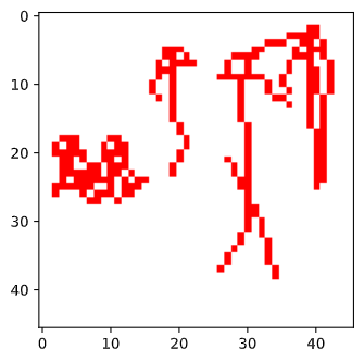
以上の処理で得られるのが,最終的な出力となる.正面の女性の右側部分のボーンが推定できていないのが不服であるが,大方予測できていることがわかる.
|
|---|
| 図15.最終出力. |
3.おわりに
本報告では,姿勢推定技術の理解を深めるため,OpenPoseの解説と実装コードを示した.論文では簡単に書かれていることが,実装では非常に複雑な処理であったり,ちょっとした誤解が致命的なバグになったり(heatmapの誤差関数の注意点参照)とかなり大変であった.
4.課題
精度はまだ粗く,実用的なものとは言い難い.精度が悪い原因は以下の3点が考えられる.
-
Iteration数が公式実装の半分
→最適解を求められていない可能性がある.
-
学習データセットが足りない
→今回はCOCO2014+2017のみを用いている.MPIIデータセットも追加して学習を回したい.
-
前処理と後処理の工夫が足りない.
→公式実装では,複数のアスペクト比を入力にあたえて,その出力の平均を取る工夫をしているが,今回の実装では,未実装である.
5.学習情報の詳細
学習情報の詳細を以下に示す.
- データセット:COCO2014+2017
- 入力サイズ:$(368,368)$
- 学習用データセット:COCO2014 train+val,COCO2017 train
- 検証用データセット:COCO2017 val
- データ拡張(詳細は省略)
- 回転($[-45^{\circ},45^{\circ}]$)
- スケール($[0.5,1.1]$)
- コントラスト($[0.5,1.5]$)
- 輝度($[-32,32]$)
- チャネル交換
- Heatmap作成
- $\sigma=7$
- PAF作成
- $\sigma_c=1$
- 学習
- Adam Optimizer
lr=1e-4, weight_decay=5e-4- 20kイテレーションごとに$\times0.5$倍
- 200kイテレーション
- Adam Optimizer
- 推定
- Heatmap Threshold: 0.3
- 線積分サンプル数:10
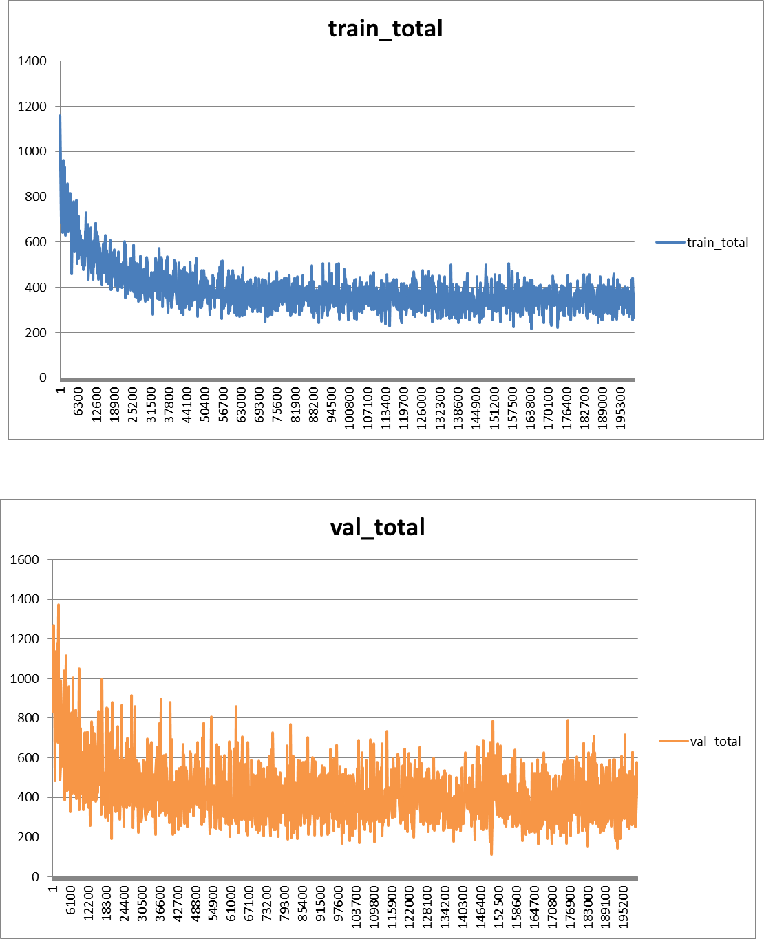 |
|---|
| 図16.学習結果. |
6.参考
-
Z. Cao et al., "OpenPose: Realtime Multi-Person 2D Pose Estimation using Part Affinity Fields", IEEE Transactions on Pattern Analysis and Machine Intelligence, 2019. ↩ ↩2 ↩3
-
Z. Cao et al., "Realtime Multi-person 2D Pose Estimation Using Part Affinity Fields," 2017 IEEE Conference on Computer Vision and Pattern Recognition (CVPR), 2017, pp.1302-1310. ↩
-
S. Liu and W. Deng, "Very deep convolutional neural network based image classification using small training sample size," 2015 3rd IAPR Asian Conference on Pattern Recognition (ACPR), 2015, pp.730-734. ↩ ↩2
-
K. He et al., "Deep Residual Learning for Image Recognition," 2016 IEEE Conference on Computer Vision and Pattern Recognition (CVPR), 2016, pp.770-778. ↩