機械学習ライブラリ「TensorFlow」と、オープンソースのシステムトレードフレームワーク「Jiji」を組み合わせて、機械学習を使った為替(FX)のトレードシステムを作るチュートリアルです。
システムのセットアップからはじめて、機械学習モデルの作成、トレーニング、それを使って実際にトレードを行うところまで、具体例を交えて解説します。
システム構成
次のようなシステムを作ります。
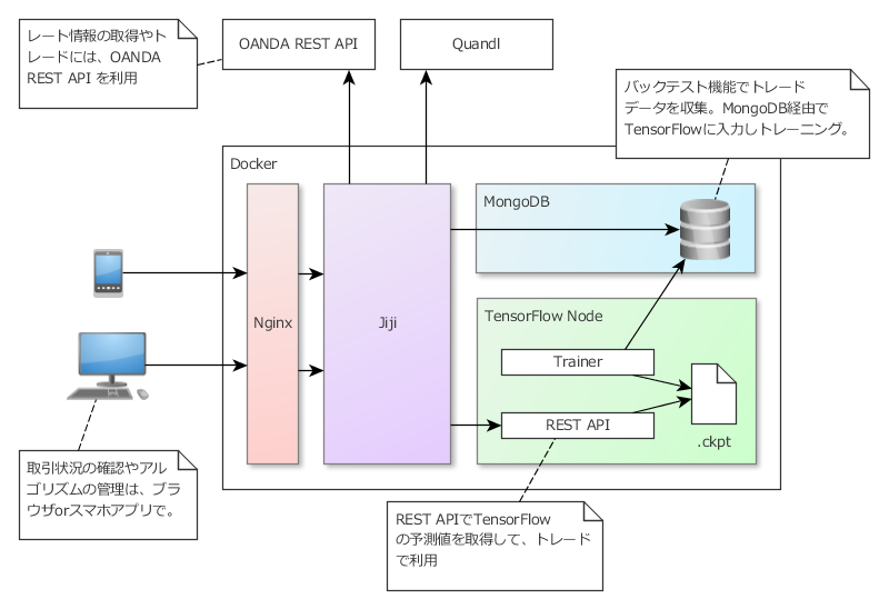
- Jijiのバックテスト機能を使ってトレードデータを収集。これをTensorFlowに入力してモデルをトレーニングします。
- 予測する内容については後述。
- 訓練したモデルを使って予測結果を返すREST APIを作り、トレード時にJijiから呼び出して使います。
- レート情報の取得やトレードには、OANDA REST API を利用
- トレード状況の確認やアルゴリズムの管理は、ブラウザ or スマホアプリで
- 外出先でも状況の確認や、緊急メンテナンスが行えるようにします。
- システムは、Docker上に構築します。
- AWSなどDockerをサポートしているクラウド環境でも、同様の手順で構築できるはずです。
- 確認はローカルマシンにインストールしたDockerで行っています。
TensorFlowで予測する内容
機械学習の使い方はいろいろ考えられると思いますが、このチュートリアルでは「トレード時の各種指標から損益を予測し、マイナスになるトレードをフィルタリングする」形での利用を試してみます。
- 移動平均の交差ルールでトレードするシンプルなアルゴリズムを作成し、トレード時の各種指標を記録。
- 記録した指標とトレードの損益データをTensorFlowに入力して学習させ、「プラス or マイナス」を予測させます。
- 予測結果が「プラス」となった場合のみトレードを行うことで、損益を改善します。
チュートリアル
順に解説していきます。
0. 前提条件
docker, docker-compose を使用します。事前にインストールをお願いします。
手順の確認は以下の環境で行っています。
- CentOS 7
- Docker 1.10.2
- Docker Compose 1.6.2
1. OANDA Japan アカウントの用意
OANDA REST API を利用するため、OANDA のアカウントが必要になります。
とりあえず試すには、無料のデモアカウントが手軽で便利です。アカウント作成はこちらから。
アカウントを作成したら、こちらの手順にしたがってパーソナルアクセストークンを発行してください。トークンはJijiの初期設定で使用します。
2. システムのセットアップ
docker-compose.yml など必要な設定ファイル/ソースコード一式は GitHub に置いています。まずはこれをダウンロード。
$ git clone https://github.com/unageanu/jiji-with-tensorflow-example.git
$ cd jiji-with-tensorflow-example
サーバー証明書の準備
通信内容を暗号化するため、TLSを使用します。
ドメインがある場合はLet’s Encrypt を利用するのが良いと思いますが、ローカルマシンなのでとりあえず自己署名証明書を使います。
$ mkdir -p ./cert
$ cd ./cert

# 秘密鍵を生成
$ openssl genrsa 2048 > server.key
# CSRを作成
$ openssl req -new -key server.key > server.csr
# サーバー証明書を作成
$ openssl x509 -sha256 -days 365 -req -signkey server.key < server.csr > server.crt
# アクセス権を制限
$ sudo chown root.root server.key
$ sudo chmod 600 server.key

$ cd ../
設定ファイルの編集
次に ./docker-compose.yml を開き、Jijiのシークレットキーを適当に変更します。
jiji:
  # 略
  environment:
    # サーバー内部で秘匿データの暗号化に使うキー
    # 必ず変更して使用してください。
    # UIから入力を求められることはないので、任意の長い文字列を使用すればOKです。
    USER_SECRET: d41d8cd98f00b204e9800998ecf8427e
システムの起動
以上で準備は完了。docker-compose でシステムを起動します。
$ docker-compose up -d
jiji_example__nginx, jiji_example__jiji, jiji_example__mongodb, jiji_example__tensorflow の各コンテナが起動していればOK。
$ docker ps -a
CONTAINER ID        IMAGE                                         COMMAND                  CREATED             STATUS                      PORTS                                                        NAMES
f083efd4ab5c        unageanu/jiji-nginx:latest                    "nginx -g 'daemon off"   8 seconds ago       Up 4 seconds                80/tcp, 0.0.0.0:10443->443/tcp                               jiji_example__nginx
ac72354363c9        unageanu/jiji:latest                          "puma -C /app/jiji2/c"   10 seconds ago      Up 8 seconds                8080/tcp                                                     jiji_example__jiji
8acc4e79e5cb        jijiwithtensorflowexample_tensorflow          "/run_jupyter.sh"        16 seconds ago      Up 10 seconds               8888/tcp, 0.0.0.0:15000->5000/tcp, 0.0.0.0:16006->6006/tcp   jiji_example__tensorflow
3e02f8b562f1        mongo:3.0.7                                   "/entrypoint.sh mongo"   20 seconds ago      Up 16 seconds               0.0.0.0:37017->27017/tcp                                     jiji_example__mongodb
Jijiの初期設定
以下のURLをブラウザで開くと、Jijiの初期設定画面が開きます。
https://<インストール先ホスト>:10443
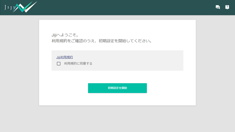
画面が表示されたら、こちらの手順に従って初期設定を行ってください。
3. トレードデータの収集
Jijiのセットアップが完了したら、トレードデータの収集に移ります。
移動平均でトレードするアルゴリズムを作り、Jijiのバックテスト機能を使って実行。このとき、「トレード損益+トレード時の各種指標」をMongoDBに記録し、これをTensorFlowの訓練データとして使います。
トレードアルゴリズム(エージェント)を作る
ソースコードはこちらにあります。主要なクラスを簡単に解説しておきます。
TradeAndSignals
- トレード結果とトレード時の各種指標を格納するクラスです。
- これをTensorFlowに入力して、トレーニングを行います。
- 指標には、移動平均の傾き/乖離率、RSI、MACDの乖離を使うようにしました。
# トレード結果とトレード時の各種指標。
# MongoDBに格納してTensorFlowの学習データにする
class TradeAndSignals

  include Mongoid::Document

  store_in collection: 'tensorflow_example_trade_and_signals'

  field :macd_difference,    type: Float # macd - macd_signal

  field :rsi,                type: Float

  field :slope_10,           type: Float # 10日移動平均線の傾き
  field :slope_25,           type: Float # 25日移動平均線の傾き
  field :slope_50,           type: Float # 50日移動平均線の傾き

  field :ma_10_estrangement, type: Float # 10日移動平均からの乖離率
  field :ma_25_estrangement, type: Float
  field :ma_50_estrangement, type: Float

  field :profit_or_loss,     type: Float
  field :sell_or_buy,        type: Symbol
  field :entered_at,         type: Time
  field :exited_at,          type: Time

  def self.create_from( signal_data, position )
    TradeAndSignals.new do |ts|
      signal_data.each do |pair|
        next if pair[0] == :ma5|| pair[0] == :ma10
        ts.send( "#{pair[0]}=".to_sym, pair[1] )
      end
      ts.profit_or_loss = position.profit_or_loss
      ts.sell_or_buy    = position.sell_or_buy
      ts.entered_at     = position.entered_at
      ts.exited_at      = position.exited_at
    end
  end
end
SignalCalculator
- シグナルを計算するクラス
- Jijiに標準添付されている
Signalsライブラリを利用してRSIや移動平均を計算します。
# シグナルを計算するクラス
class SignalCalculator

  def initialize(broker)
    @broker = broker
  end

  def next_tick(tick)
    prepare_signals(tick) unless @macd
    calculate_signals(tick[:USDJPY])
  end

  def calculate_signals(tick)
    price = tick.bid
    macd = @macd.next_data(price)
    ma5  = @ma5.next_data(price)
    ma10 = @ma10.next_data(price)
    ma25 = @ma25.next_data(price)
    ma50 = @ma50.next_data(price)
    {
      ma5:  ma5,
      ma10: ma10,
      macd_difference: macd ? macd[:macd] - macd[:signal] : nil,
      rsi:  @rsi.next_data(price),
      slope_10: ma10 ? @ma10v.next_data(ma10) : nil,
      slope_25: ma25 ? @ma25v.next_data(ma25) : nil,
      slope_50: ma50 ? @ma50v.next_data(ma50) : nil,
      ma_10_estrangement: ma10 ? calculate_estrangement(price, ma10) : nil,
      ma_25_estrangement: ma25 ? calculate_estrangement(price, ma25) : nil,
      ma_50_estrangement: ma50 ? calculate_estrangement(price, ma50) : nil
    }
  end

  def prepare_signals(tick)
    create_signals
    retrieve_rates(tick.timestamp).each do |rate|
      calculate_signals(rate.close)
    end
  end

  def create_signals
    @macd  = Signals::MACD.new
    @ma5   = Signals::MovingAverage.new(5)
    @ma10  = Signals::MovingAverage.new(10)
    @ma25  = Signals::MovingAverage.new(25)
    @ma50  = Signals::MovingAverage.new(50)
    @ma5v  = Signals::Vector.new(5)
    @ma10v = Signals::Vector.new(10)
    @ma25v = Signals::Vector.new(25)
    @ma50v = Signals::Vector.new(50)
    @rsi   = Signals::RSI.new(9)
  end

  def retrieve_rates(time)
    @broker.retrieve_rates(:USDJPY, :one_day, time - 60*60*24*60, time )
  end

  def calculate_estrangement(price, ma)
    ((BigDecimal.new(price, 10) - ma) / ma * 100).to_f
  end

end
TensorFlowSampleAgent
- トレードアルゴリズムの本体。
-
SignalCalculatorで計算した5日移動平均と10日移動平均のクロスでトレードを行います。- 5日移動平均 > 10日移動平均 の場合、買
- 5日移動平均 < 10日移動平均 の場合、売
- プロパティで、動作モードを次の3つから選べるようにしています。
-
collect: トレードデータ収集時に使います。ポジションの決済時にTradeAndSignalsをMongoDBに保存します。 -
trade: TensorFlowでの予測を使用してトレードを行うモードです。訓練後の評価で使います。 -
test: TensorFlowでの予測を使用せずトレードを行うモード。tradeモードの結果を評価する際に比較用に使用します。
-
# TensorFlowと連携してトレードするエージェントのサンプル
class TensorFlowSampleAgent

  include Jiji::Model::Agents::Agent

  def self.description
    <<-STR
TensorFlowと連携してトレードするエージェントのサンプル
      STR
  end

  def self.property_infos
    [
      Property.new('exec_mode',
        '動作モード("collect" or "trade" or "test")', "collect")
    ]
  end

  def post_create
    @calculator = SignalCalculator.new(broker)
    @cross = Cross.new
    @mode  = create_mode(@exec_mode)

    @graph = graph_factory.create('移動平均',
      :rate, :last, ['#FF6633', '#FFAA22'])
  end

  # 次のレートを受け取る
  def next_tick(tick)
    date = tick.timestamp.to_date
    return if !@current_date.nil? && @current_date == date
    @current_date = date

    signal = @calculator.next_tick(tick)
    @cross.next_data(signal[:ma5], signal[:ma10])

    @graph << [signal[:ma5], signal[:ma10]]
    do_trade(signal)
  end

  def do_trade(signal)
    # 5日移動平均と10日移動平均のクロスでトレード
    if @cross.cross_up?
      buy(signal)
    elsif @cross.cross_down?
      sell(signal)
    end
  end

  def buy(signal)
    close_exist_positions
    return unless @mode.do_trade?(signal, "buy")
    result = broker.buy(:USDJPY, 10000)
    @current_position = broker.positions[result.trade_opened.internal_id]
    @current_signal = signal
  end

  def sell(signal)
    close_exist_positions
    return unless @mode.do_trade?(signal, "sell")
    result = broker.sell(:USDJPY, 10000)
    @current_position = broker.positions[result.trade_opened.internal_id]
    @current_signal = signal
  end

  def close_exist_positions
    return unless @current_position
    @current_position.close
    @mode.after_position_closed( @current_signal, @current_position )
    @current_position = nil
    @current_signal = nil
  end

  def create_mode(mode)
    case mode
    when 'trade' then
      TradeMode.new
    when 'collect' then
      CollectMode.new
    else
      TestMode.new
    end
  end

  # データ収集モード
  #
  # TensorFlowでの予測を使用せずに移動平均のシグナルのみでトレードを行い、
  # 結果をDBに保存する
  #
  class CollectMode
    def do_trade?(signal, sell_or_buy)
      true
    end
    # ポジションが閉じられたら、トレード結果とシグナルをDBに登録する
    def after_position_closed( signal, position )
      TradeAndSignals.create_from( signal, position).save
    end
  end

  # テストモード
  #
  # TensorFlowでの予測を使用せずに移動平均のシグナルのみでトレードする
  # トレード結果は収集しない
  #
  class TestMode
    def do_trade?(signal, sell_or_buy)
      true
    end
    def after_position_closed( signal, position )
      # do nothing.
    end
  end

  # 取引モード
  #
  # TensorFlowでの予測を使用してトレードする。
  # トレード結果は収集しない
  #
  class TradeMode
    def initialize
      @client = HTTPClient.new
    end
    # トレードを勝敗予測をtensorflowに問い合わせる
    def do_trade?(signal, sell_or_buy)
      body = {sell_or_buy: sell_or_buy}.merge(signal)
      body.delete(:ma5)
      body.delete(:ma10)
      result = @client.post("http://tensorflow:5000/api/estimator", {
        body: JSON.generate(body),
        header: {
          'Content-Type' => 'application/json'
        }
      })
      return JSON.parse(result.body)["result"] == "up"
      # up と予測された場合のみトレード
    end
    def after_position_closed( signal, position )
      # do nothing.
    end
  end
end
訓練用データを取集する
エージェントができたら、Jijiのバックテスト機能を利用してアルゴリズムを実行し、トレードデータを収集します。
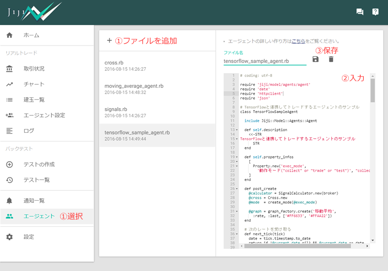
エージェントの登録
- [エージェント] 画面を開いて、「+」ボタンで新しいエージェントを追加します。
- エージェント名を「
tensorflow-sample-agent.rb」に設定、エディタに tensorflow_sample_agent.rb の内容をコピペして貼り付け。 - 最後に、保存ボタンを押して、エージェントを登録します。
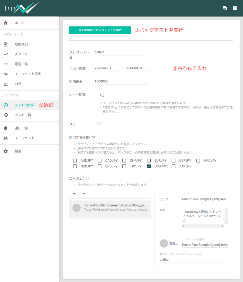
バックテストの実行
- [バックテスト] - [テストの作成] を開きます。
- テストの設定を行います。
- 「テスト名」は適当に入力。
- 過去10年のデータでテストができるので、2006~2014のトレード結果をトレーニングに使い、2014~2016はフィルタの評価に使用することにします。「テスト期間」は、2006-09-01 ~ 2014-08-31 に設定。
- 日足データのみ使用するため、「レート間隔」は「1日」にします。
- 「使用する通貨ペア」で「USDJPY」を選択
- 「エージェント」の「+」ボタンを押して、
TensorflowSampleAgent@tensorflow_sample_agent.rbを追加します。追加後、右下のプロパティで「動作モード」をcollectに設定します。
- 設定が完了したら、[以下の設定でバックテストを開始] ボタンを押して、テストを実行します。
テストの実行が完了したら、MongoDBにトレードデータが保存されているはず。接続して確認。
$ docker exec -it jiji_example__mongodb  mongo
MongoDB shell version: 3.0.7
connecting to: test
Welcome to the MongoDB shell.
> show dbs
jiji   0.203GB
local  0.078GB
> use jiji
switched to db jiji
> db.tensorflow_example_trade_and_signals.find()
{ "_id" : ObjectId("57b1593a52de170001577542"), "macd_difference" : 0.2377196586449014, "rsi" : 20.774818401937026, "slope_10" : 0.08290969696969225, "slope_25" : 0.05338855384616181, "slope_50" : null, "ma_10_estrangement" : -0.9403938769738917, "ma_25_estrangement" : -0.5138962727847769, "ma_50_estrangement" : -0.07730379529748173, "profit_or_loss" : -17860, "sell_or_buy" : "sell", "entered_at" : ISODate("2006-09-04T15:00:00Z"), "exited_at" : ISODate("2006-09-11T15:00:00Z") }
{ "_id" : ObjectId("57b1593b52de170001577549"), "macd_difference" : 0.02080019102510705, "rsi" : 60.18461538461548, "slope_10" : -0.0560551515151482, "slope_25" : 0.06835978461537653, "slope_50" : null, "ma_10_estrangement" : 0.8251919080828378, "ma_25_estrangement" : 0.8220139255524603, "ma_50_estrangement" : 1.4264079514333357, "profit_or_loss" : -4970, "sell_or_buy" : "buy", "entered_at" : ISODate("2006-09-11T15:00:00Z"), "exited_at" : ISODate("2006-09-20T15:00:00Z") }
# 略
> quit()
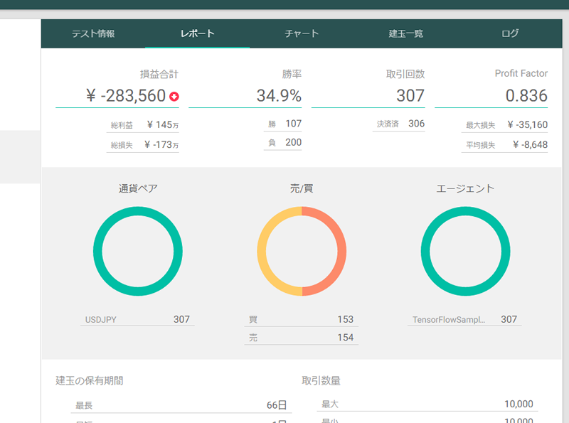
ちなみにトレード結果は以下の通りでした。シンプルなアルゴリズムなので、こんなもんですかね。
4. トレーニング
データができたので、TensorFlowのモデルをトレーニングしていきます。
訓練で必要なソースコードはコンテナ作成時にコピーしているので /scripts/train.py を実行すればOKだったりしますが、用意したコードを軽く解説しておきます。
TradeResultsLoader
- MongoDBからトレードデータを取得するクラスです。
- PyMongo を使っています。
class TradeResultsLoader:

    DB_HOST='mongodb'
    DB_PORT=27017

    DB='jiji'
    COLLECTION='tensorflow_example_trade_and_signals'

    def retrieve_trade_data(self):
        client = pymongo.MongoClient(
            TradeResultsLoader.DB_HOST, TradeResultsLoader.DB_PORT)
        collection = client[TradeResultsLoader.DB][TradeResultsLoader.COLLECTION]
        cursor = collection.find().sort("entered_at")
        return pd.DataFrame(list(cursor))
TradeResults
- トレードデータを整形するクラス。
- 以下のような処理を行います。
- データをトレーニング用とテスト用に分割。
- トレードデータの 2/3 を実際の訓練に、残りをテストデータとして訓練課程でのモデルの評価に使います。
-
z-scoreでの値の正規化 - 目的変数とする損益データを取り出して、
up,downのDataFrameに変換。
- データをトレーニング用とテスト用に分割。
class TradeResults:

    def __init__(self, data):
        self.raw  = data.copy()
        self.data = TradeResults.normalize(TradeResults.clean(data))

    def all_data(self):
        return self.__drop_profit_or_loss(self.data)

    def train_data(self):
        return self.__drop_profit_or_loss(self.__train_data())

    def test_data(self):
        return self.__drop_profit_or_loss(self.__test_data())

    def train_profit_or_loss(self):
        return self.__train_data()["normalized_profit_or_loss"]

    def test_profit_or_loss(self):
        return self.__test_data()["normalized_profit_or_loss"]

    def train_up_down(self):
        return self.__up_down(self.__train_data()["profit_or_loss"])

    def test_up_down(self):
        return self.__up_down(self.__test_data()["profit_or_loss"])

    def __train_data(self):
        # 全データの 2/3 を訓練データとして使う。
        # トレード時の地合いの影響を分散させるため、時系列でソートしたものから均等に抜き出す。
        return self.data.loc[lambda df: df.index % 3 != 0, :]

    def __test_data(self):
        # 全データの 1/3 をテストデータとして使う。
        return self.data.loc[lambda df: df.index % 3 == 0, :]

    def __drop_profit_or_loss(self, data):
        return data.drop("profit_or_loss", axis=1).drop("normalized_profit_or_loss", axis=1)

    def __up_down(self, profit_or_loss):
        return profit_or_loss.apply(
            lambda p: pd.Series([
                1 if p >  0  else 0,
                1 if p <= 0  else 0
            ], index=['up', 'down']))

    @staticmethod
    def clean(data):
        del data['_id']
        del data['entered_at']
        del data['exited_at']
        data['sell_or_buy'] = data['sell_or_buy'].apply(
            lambda sell_or_buy: 0 if sell_or_buy == "sell" else 1)
        return data

    @staticmethod
    def normalize(data):
        # すべてのデータをz-scoreで正規化する
        for col in data.columns:
            key = 'normalized_' + col if col == 'profit_or_loss' else col
            data[key] = (data[col] - data[col].mean())/data[col].std(ddof=0)
        data = data.fillna(0)
        return data
Trainer & Estimator & Model
- Modelクラスに TensorFlowのモデルを定義して、派生クラスのTrainer(訓練を行うクラス)とEstimator(予測を行うクラス)で共有する形にしています。
- モデルはコピペです。隠れ層2のシンプルなものにしてみました。
class Model:
    HIDDEN_UNIT_SIZE  = 32
    HIDDEN_UNIT_SIZE2 = 16
    COLUMN_SIZE = 9

    def __init__(self):
        self.__setup_placeholder()
        self.__setup_model()
        self.__setup_ops()

    def __enter__(self):
        self.session = tf.Session()
        return self

    def __exit__(self, exc_type, exc_value, traceback):
        self.session.close()
        return False

    def save(self, path):
        saver = tf.train.Saver()
        saver.save(self.session, path)

    def restore(self, path):
        saver = tf.train.Saver()
        saver.restore(self.session, path)

    def __setup_placeholder(self):
        column_size = Model.COLUMN_SIZE
        self.trade_data   = tf.placeholder("float", [None, column_size])
        self.actual_class = tf.placeholder("float", [None, 2])
        self.keep_prob    = tf.placeholder("float")
        self.label        = tf.placeholder("string")

    def __setup_model(self):
        column_size = Model.COLUMN_SIZE
        w1 = tf.Variable(tf.truncated_normal([column_size, Estimator.HIDDEN_UNIT_SIZE], stddev=0.1))
        b1 = tf.Variable(tf.constant(0.1, shape=[Estimator.HIDDEN_UNIT_SIZE]))
        h1 = tf.nn.relu(tf.matmul(self.trade_data, w1) + b1)

        w2 = tf.Variable(tf.truncated_normal([Estimator.HIDDEN_UNIT_SIZE, Estimator.HIDDEN_UNIT_SIZE2], stddev=0.1))
        b2 = tf.Variable(tf.constant(0.1, shape=[Estimator.HIDDEN_UNIT_SIZE2]))
        h2 = tf.nn.relu(tf.matmul(h1, w2) + b2)

        h2_drop = tf.nn.dropout(h2, self.keep_prob)
        w2 = tf.Variable(tf.truncated_normal([Estimator.HIDDEN_UNIT_SIZE2, 2], stddev=0.1))
        b2 = tf.Variable(tf.constant(0.1, shape=[2]))
        self.output = tf.nn.softmax(tf.matmul(h2_drop, w2) + b2)

    def __setup_ops(self):
        cross_entropy = -tf.reduce_sum(self.actual_class * tf.log(self.output))
        self.summary = tf.scalar_summary(self.label, cross_entropy)
        self.train_op = tf.train.AdamOptimizer(0.0001).minimize(cross_entropy)
        self.merge_summaries = tf.merge_summary([self.summary])
        correct_prediction = tf.equal(tf.argmax(self.output,1), tf.argmax(self.actual_class,1))
        self.accuracy = tf.reduce_mean(tf.cast(correct_prediction, "float"))


class Trainer(Model):

    def train(self, steps, data):
        self.__prepare_train(self.session)
        for i in range(steps):
            self.__do_train(self.session, i, data)
            if i %100 == 0:
                self.__add_summary(self.session, i, data)
                self.__print_status(self.session, i, data)

    def __prepare_train(self, session):
        self.summary_writer = tf.train.SummaryWriter('logs', graph_def=session.graph_def)
        session.run(tf.initialize_all_variables())

    def __do_train(self, session, i, data):
        session.run(self.train_op, feed_dict=self.train_feed_dict(data))

    def __add_summary(self, session, i, data):
        summary_str = session.run(self.merge_summaries, feed_dict=self.train_feed_dict(data))
        summary_str += session.run(self.merge_summaries, feed_dict=self.test_feed_dict(data))
        self.summary_writer.add_summary(summary_str, i)

    def __print_status(self, session, i, data):
        # 現在のモデルを利用して推移した利益と実際の利益の相関を、訓練データ、テストデータそれぞれで計算し出力する
        train_accuracy = session.run(self.accuracy, feed_dict=self.train_feed_dict(data))
        test_accuracy  = session.run(self.accuracy, feed_dict=self.test_feed_dict(data))
        print 'step {} ,train_accuracy={} ,test_accuracy={} '.format(
            i, train_accuracy, test_accuracy)

    def train_feed_dict(self, data):
        return {
            self.trade_data: data.train_data(),
            self.actual_class: data.train_up_down(),
            self.keep_prob: 0.8,
            self.label: "train"
        }

    def test_feed_dict(self, data):
        return {
            self.trade_data: data.test_data(),
            self.actual_class: data.test_up_down(),
            self.keep_prob: 1,
            self.label: "test"
        }

    def __reshape(self, profit_or_loss):
        return profit_or_loss.values.reshape(len(profit_or_loss.values), 1)


class Estimator(Model):

    def estimate( self, data ):
        return self.session.run(tf.argmax(self.output,1), feed_dict=self.estimate_feed_dict(data))

    def estimate_feed_dict(self, data):
        return {
            self.trade_data: data,
            self.keep_prob: 1
        }
train.py
- トレーニングをキックするスクリプトです。
-
TradeResultsLoaderを使って取得したトレードデータをTrainerに渡して訓練を行っています。 - 訓練が終わったら、モデルを
./model.ckptに永続化します。
# -*- coding: utf-8 -*-

from trade_results_loader import *
from model import *

loader = TradeResultsLoader()
data = TradeResults(loader.retrieve_trade_data())

with Trainer() as trainer:
    trainer.train(10001, data)
    trainer.save("./model.ckpt")
train.py の実行
前述のとおり、必要なスクリプトはコンテナ作成時にコピーしているので、コンテナ内で実行すれば、訓練を開始できます。
まずは、TensorFlowコンテナに入ります。
$ docker exec -it jiji_example__tensorflow /bin/bash
コンテナ内で以下を実行します。
$ cd /scripts
$ python train.py
step 0 ,train_accuracy=0.671568632126 ,test_accuracy=0.607843160629
step 100 ,train_accuracy=0.671568632126 ,test_accuracy=0.607843160629
step 200 ,train_accuracy=0.671568632126 ,test_accuracy=0.607843160629
step 300 ,train_accuracy=0.671568632126 ,test_accuracy=0.607843160629
# 略
step 9600 ,train_accuracy=0.936274528503 ,test_accuracy=0.568627476692
step 9700 ,train_accuracy=0.965686261654 ,test_accuracy=0.578431367874
step 9800 ,train_accuracy=0.946078419685 ,test_accuracy=0.558823525906
step 9900 ,train_accuracy=0.946078419685 ,test_accuracy=0.558823525906
100ステップごとに、モデルを使って訓練データを予測した時の精度と、テストデータを予測した時の精度が出力されます。
訓練は、とりあえず 10000ステップ行うようにしてみました。
最終的には以下の精度になりました。
step 9900 ,train_accuracy=0.946078419685 ,test_accuracy=0.558823525906
訓練データでの精度は高いのですが、テストデータでの精度は微妙・・・。あてずっぽうよりはましかな・・・。
5. バックテストで検証
精度に一抹の不安が残りますが、このまま突き進みます。
次は、訓練したモデルを使って予測した結果を返すREST APIを作ります。
REST API を作る
-
Estimatorで推測した結果を返す機能を、Flaskを使ってREST APIで公開します。 - リクエストボディで渡された指標データを正規化して
Estimatorに渡し、予測させた損益結果(upordown)を返却します。- データの正規化に訓練時に使用したデータが必要なので、
TradeResultsLoaderでトレードデータを取得して、TradeResultsで正規化する処理を入れています。
- データの正規化に訓練時に使用したデータが必要なので、
loader = TradeResultsLoader()

estimator = Estimator()
estimator.__enter__()
estimator.restore("./model.ckpt")

trade_data  = loader.retrieve_trade_data()

# webapp
app = Flask(__name__)

@app.route('/api/estimator', methods=['POST'])
def estimate():
    # 値を正規化するため、リクエストボディで渡された指標データと訓練で使用したデータを統合。
    data = pd.DataFrame({k: [v] for k, v in request.json.items()}).append(trade_data)
    # 正規化したデータを渡して、損益を予測
    results = estimator.estimate(TradeResults(data).all_data().iloc[[0]])
    return jsonify(result=("up" if results[0] == 0 else "down"))

if __name__ == '__main__':
    app.run(host='0.0.0.0')
サーバーのソースコードもコンテナにコピーしているので、以下のコマンドでサーバーを起動できます。
$ cd /scripts
$ python server.py
フィルタの効果検証
REST APIができたので、Jijiのトレードアルゴリズムから実際に使用してフィルタの効果を検証します。
- 訓練には2006~2014の結果を利用したので、2014~2016 の期間で効果を検証します。
- TensorFlowの予測を使用しない
testモードでのトレード結果と、予測を使用するtradeモードでそれぞれバックテストを行い結果を比較します。
まずは、test モードで実行。
- [バックテスト] - [テストの作成] を開きます。
- テストの設定を行います。
- 「テスト名」は適当に入力。
- 「テスト期間」は、2014-09-01 ~ 2016-08-01 に設定。
- 「レート間隔」は「1日」にします。
- 「使用する通貨ペア」で「USDJPY」を選択
- 「エージェント」の「+」ボタンを押して、
TensorflowSampleAgent@tensorflow_sample_agent.rbを追加します。追加後、右下のプロパティで「動作モード」をtestに設定します。
- 設定が完了したら、[以下の設定でバックテストを開始] ボタンを押して、テストを実行します。
フィルタなしの場合のトレード結果は以下の通りでした。
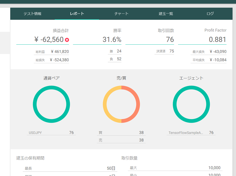
同様の設定で、動作モードを trade にして再度テストを実行。TensorFlow フィルタが適用されます。
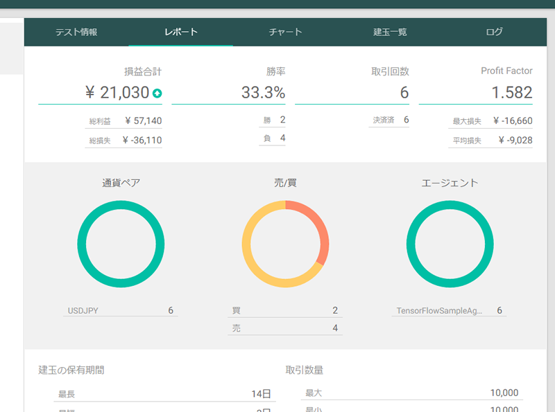
うーん、微妙。損益とProfit Factorは改善していますが、トレード回数が大幅減・・・。トレードしていないわけではないので、すべて「マイナス」と判定している訳ではなそさそうですが、「マイナス」寄りに大きく傾いている気がしますね・・・。
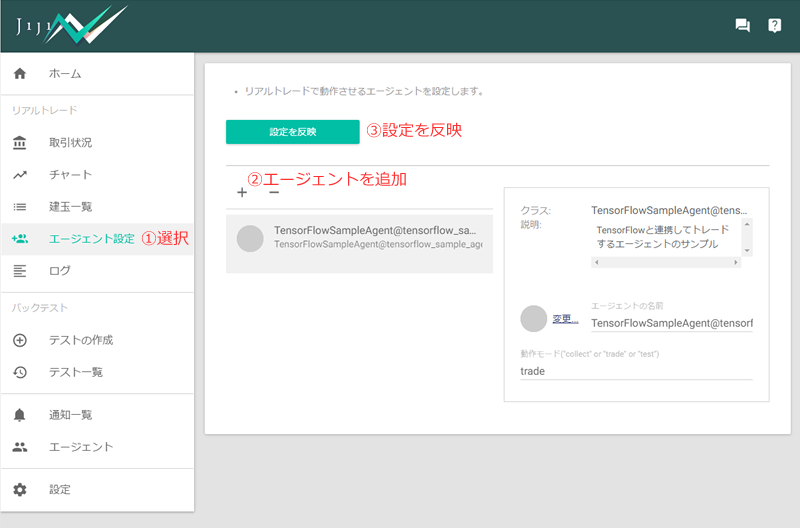
6. アルゴリズムを使って実際の口座でトレード
最後に、一応、アルゴリズムを使って実際の口座でトレードするところまで解説しておきます。といっても、アルゴリズム(エージェント)を [リアルトレード]-[エージェント]に登録するだけですが。
登録すれば、実際の口座(個人口座orデモ口座)でアルゴリズムの運用を開始できます。
もちろん、事前に十分な動作確認を行ってくださいね。
まとめ
チュートリアルは以上です。
フィルタとしての効果は微妙でしたが、説明変数として渡すデータやモデルの設定を調整すれば改善できる余地はあるかもしれません。また、そもそも、ベースとしている移動平均を使ったトレードアルゴリズムの予測能力も低いので、これをもっと良いものに変えることで結果を良くすることができる可能性もあります。興味がある方は、環境を作っていろいろ試してみてください。
TensorFlowのような機械学習ライブラリやOANDA REST APIの登場で、個人でも手軽に先端技術を利用したシステムトレードを試せる環境が整ってきているように思います。データ分析や機械学習の勉強も兼ねて、システムトレードに取り組んでみるのも面白いのではないでしょうか?