金利曲線をモデリングするために、1987年にCharles R. NelsonとAndrew F. SiegelはNelson-Siegelモデルを提唱しました。特に、このモデルはゼロクーポンボンドのイールドカーブを表現するのに適しています。様々な計算手法が提案されています。ここでは単純な方法で計算していますが、状態空間方程式を用いたものも多数報告されています。またストラング先生の5版のIntroduction to Linear Algebraで紹介されている主成分分析を用いたものもあります。ここでの説明は初歩的なものであり、コメントをいただけると助かります。
コードは
https://github.com/innovation1005/qiita_innovation1005
にアップしてあります。
Nelson-Siegelモデルは以下の式で表されます。
$$Y(t) = b_0 + b_1 * [(1 - \exp(-t/\tau)) / (t/\tau)] + b_2 * {[(1 - \exp(-t/\tau)) / (t/\tau)] - \exp(-t/\tau)}$$
ここで、
$Y(t)$ は満期までの時間 t のゼロクーポンボンドのイールドを表します。
$b_0$, $b_1$, $b_2$ はモデルのパラメータで、イールドカーブの水準(level)、傾き(slope)、および曲率(curvature)を表します。
$\tau$ はスケーリングパラメータで、カーブの形状を調整します。
モデルの特徴は、これら3つの要素を使用して金利曲線を捉えることです。
水準・レベル($b_0$)は、長期的なイールド(時間が無限大に近づくときのイールド)を反映します。
傾き($b_1$)は短期と長期のイールドとの間のスプレッド(金利差)を表します。
曲率($b_2$)は中期のイールドの動きを表します。
Nelson-Siegelモデルは金利モデルの基礎となっています。
import pandas as pd
import matplotlib.pyplot as plt
import numpy as np
import statsmodels.api as sm
from statsmodels.tsa.arima.model import ARIMA
from statsmodels.api import OLS
from pandas.tseries.offsets import DateOffset

import pandas_datareader.data as web
start="1949/5/16"
金利のデータをFREDから入手します。
10-Year Treasury Constant Maturity Rate (DGS10) daily
5-Year Treasury Constant Maturity Rate (DGS5) daily
1-Year Treasury Constant Maturity Rate (DGS1) daily
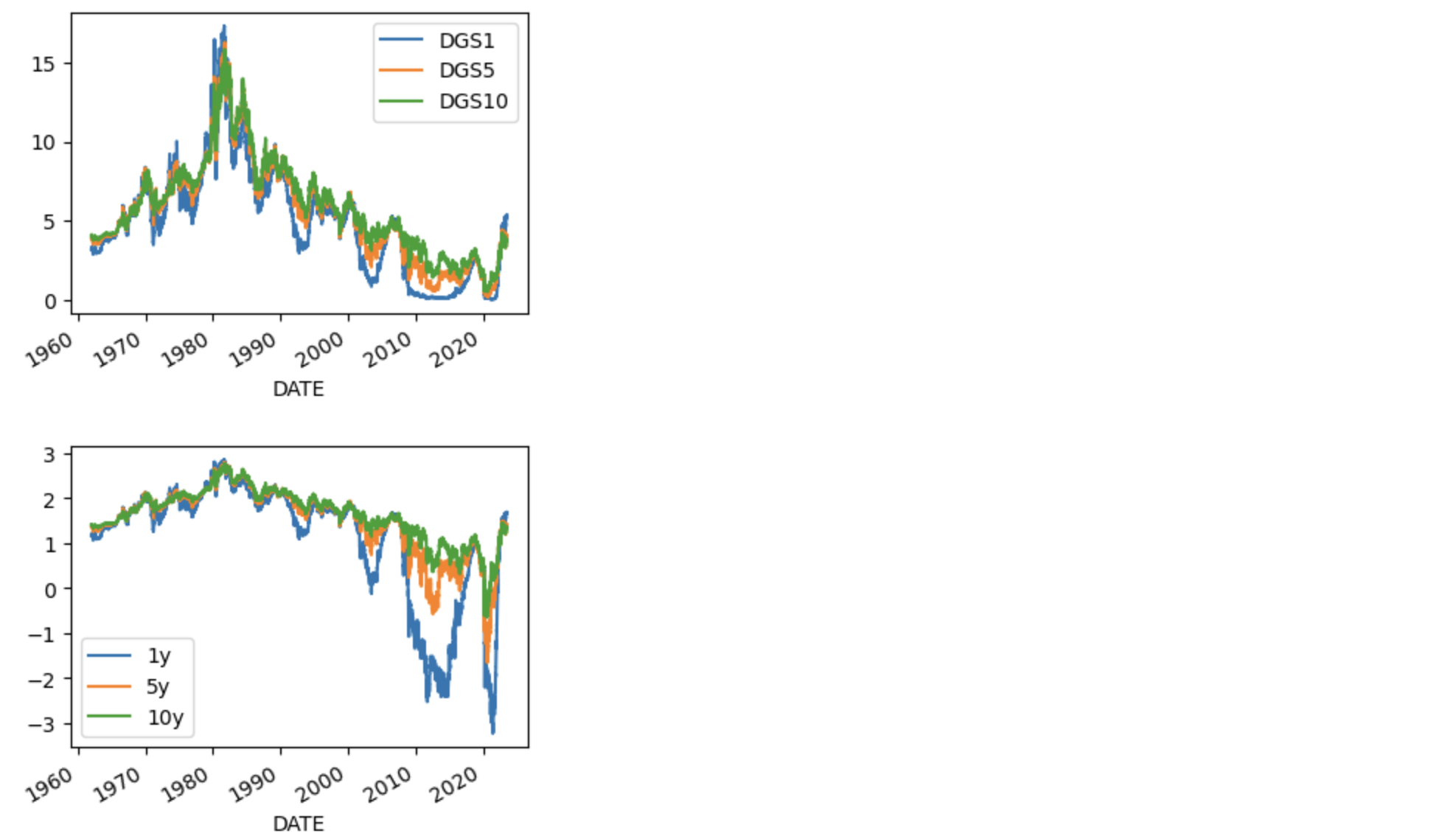
モデルを簡単にするために、3つの満期の米国財務省債券のConstant Maturity Rate(CMR)を使います。ゼロカーブは使いません。また長期の金利なので対数を取ってみました。
ty10 = web.DataReader("DGS10", 'fred',start)#Population, Total for World
ty5 = web.DataReader("DGS5", 'fred',start)#Population, Total for World
ty1 = web.DataReader("DGS1", 'fred',start)#Population, Total for World
ty=pd.concat([ty1,ty5,ty10],axis=1).dropna()

ty.plot(figsize=(4,3))
ty.columns=['1y','5y','10y']
plt.show()
lnty=np.log(ty)
lnty.plot(figsize=(4,3))
plt.show()
水準、傾き、曲率の3パラメータの算出
Nelson-Siegelモデルの米国債のイールドカーブを3つの満期のCMRから構築します。日足のデータが手に入るので、3つのCRMを水準、傾き、曲率の3つの変数で説明するモデルを最小二乗法を用いて求めます。つまり水準、傾き、曲率の係数は日々計算します。
# Nelson-Siegel model shape functions
def ns_shape_0(t, lambda_):
    return np.ones_like(t)

def ns_shape_1(t, lambda_):
    return (1 - np.exp(-lambda_*t)) / (lambda_*t)

def ns_shape_2(t, lambda_):
    return ((1 - np.exp(-lambda_*t)) / (lambda_*t)) - np.exp(-lambda_*t)
t_values = np.array([1, 5, 10])

# Choose a value for the shape parameter lambda
lambda_ = 0.1
endog=lnty
# Perform the linear regression to estimate b0, b1, b2 for each time point
X=[]
for t in endog.index:
    # Calculate the values of the shape functions for each maturity
    shape_0_values = ns_shape_0(t_values, lambda_)
    shape_1_values = ns_shape_1(t_values, lambda_)
    shape_2_values = ns_shape_2(t_values, lambda_)

    # Create a DataFrame with the shape function values
    shape_df = pd.DataFrame({
        'shape_0': shape_0_values,
        'shape_1': shape_1_values,
        'shape_2': shape_2_values,
    }, index=['1y', '5y', '10y'])

    y = endog.loc[t, :]
    model = OLS(y, shape_df)
    results = model.fit()
    #estimated_params.loc[t,['b0', 'b1', 'b2']] = results.params.values
    X.append(results.params.values)

X=pd.DataFrame(X,index=endog.index,columns=['b0','b1','b2'])
plt.plot(X)
plt.show()
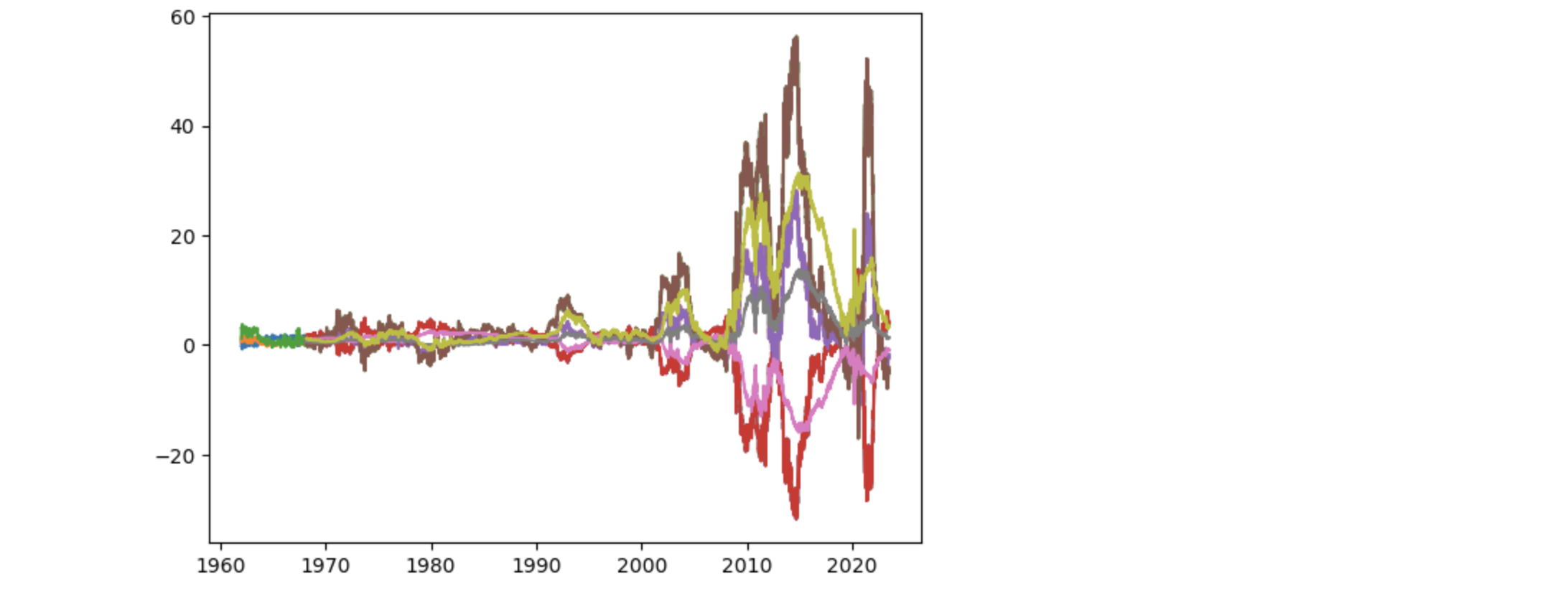
3つのパラメータを時系列データとしてプロットします。
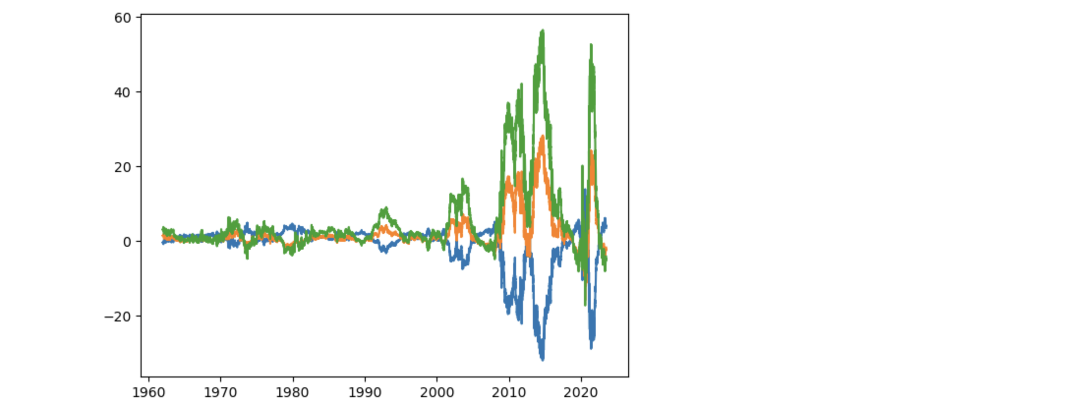
対数を取っているので、金利の動きとは異なり、金利は1980年の前半でピークをつくりその後下落します。対数のグラフも同様ですが、その上下動の大きさに違いがあります。3つのパラメータを時系列データとして表現したとき、2000年を境にその上下動が大きくなります。
3パラメータの予測
パラメートの予測モデルを作ります。3つのパラメータの推移を時系列データとして扱い、1期前の金利の係数分と乱数がつぎの期の金利に反映される1次の自己回帰モデルを用いて、これら3つのパラメータを表現します。
def forecastARIMA(nforecasts,X=X['b0'],order=(1,0,0)):
endog=X.copy()
da=[]
fv=[]
f = []
f250=[]
if not isinstance(endog.index, pd.PeriodIndex):
endog.index = endog.index.to_period('D') # ここでは日次データを仮定しています
# Get the number of initial training observations
nobs = len(endog)
n_init_training = int(nobs * 0.1)
nobs2=n_init_training
# Create model for initial training sample, fit parameters
training_endog = endog.iloc[:n_init_training]
mod = ARIMA(training_endog, order=order)
res = mod.fit(method='yule_walker')
# Save initial forecast
da.append(training_endog.index[-1])
fv=res.fittedvalues.values.tolist()
f.append(res.forecast(steps=nforecasts).values[-1])
f250.append(res.forecast(steps=250).values[-1])
#print(len(fv),fv)
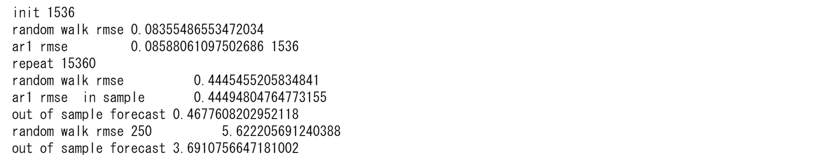
print('init',n_init_training)
print('random walk rmse', training_endog.diff().var()**0.5)
print('ar1 rmse ',(np.mean(res.resid**2))**0.5,len(res.resid))
# Step through the rest of the sample
for t in range(n_init_training, nobs):
# Update the results by appending the next observation
updated_endog = endog.iloc[t-nobs2:t+1]
mod = ARIMA(updated_endog,order=order)
res = mod.fit(method='yule_walker')
# Save the new set of forecasts
da.append(updated_endog.index[-1])
fv.append(res.fittedvalues.values[-1])
f.append(res.forecast(steps=nforecasts).values[-1])
f250.append(res.forecast(steps=250).values[-1])
print('repeat',nobs)
print('random walk rmse ', endog.diff().var()**0.5)
fv=pd.DataFrame(fv,index=X.index,columns=["fv"])
print('ar1 rmse in sample ',(np.mean((fv.values.T-endog.values.T)**2)**0.5,len(res.resid))[0])
fc=pd.DataFrame(f,index=X.index[-len(f):],columns=['fc'])
tmp=pd.concat([fc,endog],axis=1).dropna()
tmp.columns=['fc','ny']
# ここでは日次データを仮定しています,
print("out of sample forecast", np.mean((fc.iloc[:-1].T.values-endog.iloc[-len(fc)+1:].T.values)**2)**0.5)
print('random walk rmse 250 ', endog.diff(250).var()**0.5)
fc250=pd.DataFrame(f250,index=X.index[-len(f250):],columns=["fc250"])
print("out of sample forecast",np.mean((fc250.iloc[:-1].T.values-endog.iloc[-len(fc250)+1:].T.values)**2)**0.5)
return fv,fc, fc250
水準の予測
b0,b0f,b0f_250=forecastARIMA(nforecasts = 1,X=X['b0'],order=(1,0,0))

ランダムウォークの基準に比べ長期の予測にかなりの改善がみられることが分かります。
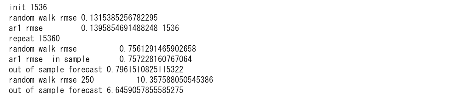
傾きの予測
b1,b1f,b1f_250=forecastARIMA(nforecasts = 1,X=X['b1'],order=(1,0,0))
ランダムウォークの基準に比べ長期の予測にかなりの改善がみられることが分かります。
曲率の予測
b2,b2f,b2f_250=forecastARIMA(nforecasts = 1,X=X['b2'],order=(1,0,0))
今まで結果をグラフにしてみます。
X = pd.DataFrame({'b0': b0.values.T[0], 'b1': b1.values.T[0], 'b2': b2.values.T[0]},index=X.index[-len(b0):])
plt.plot(X)
Xf = pd.DataFrame({'b0': b0f.values.T[0], 'b1': b1f.values.T[0], 'b2': b2f.values.T[0]},index=X.index[-len(b0f):])
plt.plot(Xf)
Xf250=pd.DataFrame({'b0': b0f_250.values.T[0], 'b1': b1f_250.values.T[0], 'b2': b2f_250.values.T[0]},index=X.index[-len(b0f_250):])
plt.plot(Xf250)
plt.show()
3パラメータからのイールドカーブの予測
3つのパラメータの推定値から元の金利の1期先、250期先を予測します。
def NS2(endog,exog,fcst,fcst250):
    # Get the number of initial training observations
    da=[]
    fv=[]
    f = []
    f250=[]
    nobs = len(endog)
    n_init_training = len(endog)-len(fcst)
    nobs2=n_init_training
    # Create model for initial training sample, fit parameters
    training_endog = endog.iloc[:n_init_training]
    training_exog = exog.iloc[:n_init_training]
    mod = OLS(training_endog.values, sm.add_constant(training_exog.values))
    res = mod.fit()
    # Save initial forecast
    da.append(training_endog.index.date[0])
    fv=res.fittedvalues.tolist()
    f.append(res.predict(sm.add_constant(training_exog).values)[0])
    f250.append(res.predict(sm.add_constant(fcst250.iloc[:n_init_training]).values)[0])

    print('init',n_init_training, 'nobs',nobs)
    print('random walk rmse', training_endog.diff().var()**0.5)
    print('ar1 rmse        ',(np.mean(res.resid**2))**0.5,len(res.resid))

    for t in range(n_init_training, nobs):
        # Update the results by appending the next observation
        updated_endog = endog.iloc[t-nobs2:t+1]
        updated_exog  =  exog.iloc[t-nobs2:t+1]
        mod = OLS(updated_endog.values, sm.add_constant(updated_exog.values))
        res = mod.fit()
        # Save the new set of forecasts
        da.append(updated_endog.index.date[-1])
        fv.append(res.fittedvalues[-1])
        fX=fcst.values[t-nobs2]
        fX= np.hstack((1, fX))
        f.append(res.predict(fX)[0])
        fX250=fcst250.values[t-nobs2]
        fX250= np.hstack((1, fX250))
        f250.append(res.predict(fX250)[0])
    fv=pd.DataFrame(fv,index=X.index)
    fc=pd.DataFrame(f,index=da)
    fc250=pd.DataFrame(f250,index=da)
    plt.plot(endog)
    plt.plot(fc,label="forecast")
    plt.plot(fc250.shift(250))
    plt.legend()
    #print(len(endog),len(f),len(f250),f)
    print('random walk rmse      ', endog.diff().var()**0.5)
    print('in sample             ',(np.mean((fv.values.T-endog.values.T)**2)**0.5,len(res.resid))[0])
    print('out of sample         ',np.mean((fc.iloc[:-1].T.values-endog.iloc[-len(fc)+1:].T.values)**2)**0.5)
    print('random walk rmse 250  ', endog.diff(250).var()**0.5)
    print('out of sample         ',np.mean((fc250.iloc[:-1].T.values-endog.iloc[-len(fc250)+1:].T.values)**2)**0.5)

print(len(ty),len(X),len(Xf),len(Xf250))
ty0=ty['1y'].iloc[-len(X):]
NS2(endog=ty['1y'].iloc[-len(X):],exog=X,fcst=Xf,fcst250=Xf250)

ここでもランダムウォークの二乗平均平方根誤差よりも予測はいい結果を示しています。グリーンの線は250日先の予測です。

このようなモデルは状態空間表現を用いて、動的なモデルで表現することもでき、それは最近のはやりです。
Python3ではじめるシステムトレード【第2版】環境構築と売買戦略

「画像をクリックしていただくとpanrollingのホームページから書籍を購入していただけます。