
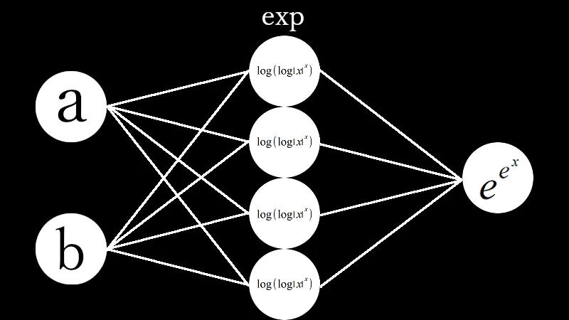
深層学習の形式で対数関数のパーセプトロンを考えてみました。
I explored a perceptron using logarithmic functions in a deep learning framework.
重みを
Let the weights be as follows:
w[0]
=
\begin{pmatrix}
1 & -1 & 0 & 0\\
0 & 0 & 1 & -1
\end{pmatrix}

w[1]
=
\begin{pmatrix}
0.5\\
0.5\\
0.5\\
-0.5
\end{pmatrix}
とし
Using these weights, we obtain the following.
入力値とw[0]の積
Product of the input and w[0]
\begin{aligned}
\begin{pmatrix}
a & b
\end{pmatrix}
\begin{pmatrix}
1 & -1 & 0 & 0\\
0 & 0 & 1 & -1
\end{pmatrix}
=
\begin{pmatrix}
a & -a & b & -b
\end{pmatrix}
\end{aligned}
中間層入力
Hidden layer input
\begin{aligned}
&
\begin{pmatrix}
log(log|a|^a) & log(log(|a|^{−a})) & log(log|b|^b) & log(log(|b|^{−b}))
\end{pmatrix}
\\
=&
\begin{pmatrix}
log(alog|a|) & log(-alog|a|) & log(blog|b|) & log(-blog|b|))
\end{pmatrix}
\end{aligned}
中間層出力とw[1]の積
Product of the hidden layer output and w[1]
\begin{aligned}
&
\begin{pmatrix}
log(alog|a|) & log(-alog|a|) & log(blog|b|) & log(-blog|b|))
\end{pmatrix}
\begin{pmatrix}
0.5\\
0.5\\
0.5\\
-0.5
\end{pmatrix}
\\
=&
0.5log(alog|a|) + 0.5log(-alog|a|) + 0.5log(blog|b|) - 0.5log(-blog|b|)
\\
=&
0.5\log\left(a\log\lvert a\rvert\right)
+
0.5\log\left(\frac{\log\lvert a\rvert}{a}\right)
+
0.5\log\left(b\log\lvert b\rvert\right)
-
0.5\log\left(\frac{\log\lvert b\rvert}{b}\right)
\end{aligned}
出力層入力
Output layer input
\begin{aligned}
&\exp\left(
  \exp\left(
    0.5\log\left(a\log\lvert a\rvert\right)
    +
    0.5\log\left(\frac{\log\lvert a\rvert}{a}\right)
    +
    0.5\log\left(b\log\lvert b\rvert\right)
    -
    0.5\log\left(\frac{\log\lvert b\rvert}{b}\right)
  \right)
\right)
\\[6pt]
={}&
\exp\left(
  \exp\left(
    0.5\log\left(
      a\log\lvert a\rvert
      \cdot
      \frac{\log\lvert a\rvert}{a}
    \right)
    +
    0.5\log\left(
      \frac{
        b\log\lvert b\rvert
      }{
        \frac{\log\lvert b\rvert}{b}
      }
    \right)
  \right)
\right)
\\[6pt]
={}&
\exp\left(
  \exp\left(
    0.5\log\left(
      \left(\log\lvert a\rvert\right)^2
    \right)
    +
    0.5\log\left(b^2\right)
  \right)
\right)
\\[6pt]
={}&
\exp\left(
  \exp\left(
    \log\left(\log a\right)
    +
    \log b
  \right)
\right)
\\[6pt]
={}&
\exp\left(
  \exp\left(
    \log\left(b\log a\right)
  \right)
\right)
\\[6pt]
={}&
\exp\left(
  b\log a
\right)
\\[6pt]
={}&
a^b
\end{aligned}
最も簡単な場合、上記条件を満たせば$a^b$を出力することができます。
In the simplest case, the network can output $a^b$ if the conditions above are satisfied.
初期値を乱数(-1.0~1.0)で決めてから学習を繰り返すと目標値に収束するか試してみました。
I tested whether repeated training would converge to the target values after initializing the weights with random values between -1.0 and 1.0.
結論から言いますと失敗しました。
To state the result up front, the attempt failed.
# coding=utf-8
import numpy as np
import matplotlib.pyplot as plt

# Initial values
# Number of training iterations
N = 10000
# Layer sizes
layer = [2, 4, 1]
# Biases
#bias = [0.0, 0.0]
# Learning rate
η = [0.01, 0.01]
#η = [0.000001, 0.000001]
# Clipping threshold
clip = 700
# Prevent overflow in exp(exp(x))
exp_clip = 6.0
# Prevent log(0) and division by zero
eps = 1.0e-12
# Number of hidden layers
H = len(η) - 1
# Target values
t = [None for _ in range(N)]
# Function output values
f_out = [[None for _ in range(H + 1)] for _ in range(N)]
# Function input values
f_in = [[None for _ in range(H + 1)] for _ in range(N)]
# Weights
w = [[None for _ in range(H + 1)] for _ in range(N + 1)]
for h in range(H):
    # The weights themselves are real-valued
    w[0][h] = np.random.uniform(-1.0, 1.0, (layer[h + 1], layer[h]))
w[0][H] = np.zeros((layer[H + 1], layer[H]))

for h in range(H + 1):
    print(w[0][h])

# Squared error
dE = [None for _ in range(N)]
#∂E/∂IN
δ = [[None for _ in range(H + 1)] for _ in range(N)]

# Training
for n in range(N):

    # Input values
    f_out[n][0] = np.random.uniform(1.2, 5.0, (layer[0]))
    f_out[n][0] = np.array(f_out[n][0], dtype=float)

    # Target values
    t[n] = np.power(f_out[n][0][0], f_out[n][0][1])

    # Reject samples only when the target value is too large
    # Allow negative hidden layer values by using complex logarithms
    while t[n] > 6.0:
        f_out[n][0] = np.random.uniform(1.2, 5.0, (layer[0]))
        f_out[n][0] = np.array(f_out[n][0], dtype=float)

        # Target values
        t[n] = np.power(f_out[n][0][0], f_out[n][0][1])

    # Forward propagation
    f_in[n][0] = np.dot(w[n][0], f_out[n][0])

    # Allow negative values by using complex logarithms
    q = f_in[n][0] * np.log(np.abs(f_in[n][0]) + eps)
    q = np.where(np.abs(q) < eps, eps + 0.0j, q)
    f_out[n][1] = np.log(np.array(q, dtype=np.complex128))

    f_in[n][1] = np.dot(w[n][1], f_out[n][1])

    # Prevent overflow in exp(exp(x))
    # Preserve the imaginary part and clip only the real part to a safe range
    f_in[n][1] = (
        np.clip(np.real(f_in[n][1]), -10.0, exp_clip)
        + 1.0j * np.imag(f_in[n][1])
    )

    # Output value
    exp = np.exp(np.exp(f_in[n][1]))

    # Derivative of the squared error with respect to the output
    dE[n] = exp - t[n]

    #δ
    δ[n][1] = exp * np.exp(f_in[n][1]) * dE[n]
    δ[n][1] = np.nan_to_num(δ[n][1])
    δ[n][1] = (
        np.clip(np.real(δ[n][1]), -clip, clip)
        + 1.0j * np.clip(np.imag(δ[n][1]), -clip, clip)
    )

    # Avoid division by zero
    safe_in = np.where(
        np.abs(f_in[n][0]) < eps,
        eps,
        f_in[n][0]
    )
    safe_log_abs = np.log(np.abs(safe_in) + eps)
    safe_log_abs = np.where(
        np.abs(safe_log_abs) < eps,
        eps,
        safe_log_abs
    )

    δ[n][0] = (
        (
            (1.0 / safe_in)
            +
            (1.0 / (safe_in * safe_log_abs))
        )
        * np.dot(w[n][1].T, δ[n][1])
    )
    δ[n][0] = np.nan_to_num(δ[n][0])
    δ[n][0] = (
        np.clip(np.real(δ[n][0]), -clip, clip)
        + 1.0j * np.clip(np.imag(δ[n][0]), -clip, clip)
    )

    # Backpropagation
    for h in range(H + 1):
        # Internal computations are complex-valued, but weight updates use only the real parts
        w[n + 1][h] = (
            w[n][h]
            -
            η[h]
            * np.real(
                δ[n][h].reshape(len(δ[n][h]), 1)
                * f_out[n][h]
            )
        )

        # Keep the weights real-valued
        w[n + 1][h] = np.real(np.nan_to_num(w[n + 1][h]))

# Output
# Values
for h in range(H + 1):
    print(w[N][h])

# Plot
# Number of subplot rows
py = np.amax(layer)
# Number of subplot columns
px = (H + 1) * 2
# Figure size
plt.figure(figsize=(16, 9))
# Horizontal axis values
x = np.arange(0, N + 1, 1)

# Draw plots
for h in range(H + 1):
    for l in range(layer[h + 1]):
        # Subplot position
        plt.subplot(py, px, px * l + h * 2 + 1)
        for m in range(layer[h]):
            # Plot only the real parts of the weights
            plt.plot(
                x,
                np.array([
                    np.real(w[n][h][l, m])
                    for n in range(N + 1)
                ]),
                label=(
                    "w["
                    + str(h)
                    + "]["
                    + str(l)
                    + ","
                    + str(m)
                    + "]"
                )
            )

        # Grid lines
        plt.grid(True)
        # Legend
        plt.legend(
            bbox_to_anchor=(1, 1),
            loc="upper left",
            borderaxespad=0,
            fontsize=10
        )

# Save the figure
plt.savefig("graph_exp_complex_real_weight.png")
# Display the figure
plt.show()

初期値
Initial values
w[0]
=
\begin{pmatrix}
-0.88835988 & 0.62603966 & -0.89836231 & -0.81327145\\
0.92129183 & -0.24692692 & 0.7553683 & 0.76288981
\end{pmatrix}

w[1]
=
\begin{pmatrix}
0\\
0\\
0\\
0
\end{pmatrix}
計算値
Computed values
w[0]
=
\begin{pmatrix}
-4.71306387 & 1.57961634 & 1.44823768 & -1.50373284\\
-1.47390817 & 1.15157137 & 3.5066877 & 0.00831848
\end{pmatrix}

w[1]
=
\begin{pmatrix}
-0.7177795\\
-0.92178776\\
-1.56781214\\
-0.28083856
\end{pmatrix}
目標値
Target values
w[0]
=
\begin{pmatrix}
1 & -1 & 0 & 0\\
0 & 0 & 1 & -1
\end{pmatrix}

w[1]
=
\begin{pmatrix}
0.5\\
0.5\\
0.5\\
-0.5
\end{pmatrix}
問題点をAIに相談したところ
When I asked an AI about the problems, it identified the following issues:
・複素対数の枝が不連続に変化する。
・The branch of the complex logarithm changes discontinuously.
・複素数の内部計算に対して、実部だけを使った更新は厳密な勾配降下法ではない。
・When internal computations involve complex numbers, updating the weights using only the real parts is not strictly gradient descent.
・中間層が 0、絶対値=1 付近で勾配が発散する。
・The gradients diverge when the hidden layer inputs approach 0 or have an absolute value close to 1.
・出力層の exp(exp(x)) が極端に不安定である。
・The output layer's exp(exp(x)) is extremely unstable.
これらの問題点があり考え直しました。
These issues led me to reconsider the approach.
改善
Improvements
元の活性化関数では、負入力に対して
For a negative input, the original activation function gives
\log\left(\log\left(|-a|^{-a}\right)\right)
=
\log(-a\log a)
となり、
which is not equal to
\log\left(\frac{\log a}{a}\right)
にはなりません。そのため、元の式をそのまま計算すると a^b ではなく a^a になります。
Therefore, evaluating the original expression as written gives a^a rather than a^b.
そこで、共通活性化関数を
I therefore defined the shared activation function as
g(z)
=
\log\left(
|z|^{\operatorname{sgn}(z)}
\log|z|
\right)
すなわち
or equivalently,
g(z)
=
\operatorname{sgn}(z)\log|z|
+
\log(\log|z|)
としました。
This is the activation function used below.
\begin{aligned}
g(a)
&=
\log(a\log a),
\\
g(-a)
&=
\log\left(\frac{\log a}{a}\right),
\\
g(b)
&=
\log(b\log b),
\\
g(-b)
&=
\log\left(\frac{\log b}{b}\right).
\end{aligned}
したがって、
It follows that
\begin{aligned}
q
&=
\frac{1}{2}g(a)
+
\frac{1}{2}g(-a)
+
\frac{1}{2}g(b)
-
\frac{1}{2}g(-b)
\\
&=
\log(\log a)+\log b
\\
&=
\log(b\log a).
\end{aligned}
最後に、
Finally,
p
=
\exp(\exp(q))
=
\exp(b\log a)
=
a^b
となります。
This gives the desired result.
最も簡単な場合、上記条件を満たせば$a^b$を出力することができます。
In the simplest case, the network can output $a^b$ if the conditions above are satisfied.

# coding=utf-8
import numpy as np
import matplotlib.pyplot as plt

# Initial values
# Number of training iterations
N = 10000
# Layer sizes
layer = [2, 4, 1]
# Batch size
batch_size = 100
# Learning rate
eta_0 = 0.0001
# Coefficient of the loss that encourages convergence to the specified matrices
matrix_loss_weight = 100.0
# Number of hidden layers
H = len(layer) - 2
# Random number generator (for reproducible random initialization)
rng = np.random.default_rng(31342)

# Training range: use a,b > 1 to evaluate the shared activation function over the reals
a_min = np.e
a_max = 10.0
b_min = np.e
b_max = 10.0

# Target weights
# This NumPy code uses weights arranged for left-multiplication of column vectors,
# so these are the transposes of the matrices shown earlier.
w_target = [None for _ in range(H + 1)]
w_target[0] = np.array([
    [1.0, 0.0],
    [-1.0, 0.0],
    [0.0, 1.0],
    [0.0, -1.0]
], dtype=np.float64)
w_target[1] = np.array([
    [0.5, 0.5, 0.5, -0.5]
], dtype=np.float64)

# Weight history
w = [[None for _ in range(H + 1)] for _ in range(N + 1)]

# Initialize all eight elements of w[0][0] with nonzero random values.
# Use the same sign within each row to keep hidden layer inputs from crossing zero.
main_weight = rng.uniform(0.55, 1.65, 4)
cross_weight = rng.uniform(0.05, 0.35, 4)
w[0][0] = np.array([
    [main_weight[0], cross_weight[0]],
    [-main_weight[1], -cross_weight[1]],
    [cross_weight[2], main_weight[2]],
    [-cross_weight[3], -main_weight[3]]
], dtype=np.float64)

# Initialize the four output layer weights with random values as well.
w[0][1] = rng.uniform(-0.8, 0.8, (layer[2], layer[1]))

for h in range(H + 1):
    print('Initial w[' + str(h) + ']')
    print(w[0][h])

# Function input and output values
f_in = [None for _ in range(H + 1)]
f_out = [None for _ in range(H + 1)]

# Loss history
loss_save = np.empty(N, dtype=np.float64)
function_loss_save = np.empty(N, dtype=np.float64)
matrix_loss_save = np.empty(N, dtype=np.float64)


def common_activation(z):
    """Activation function shared by all four neurons."""
    abs_z = np.abs(z)
    return np.sign(z) * np.log(abs_z) + np.log(np.log(abs_z))


def common_activation_derivative(z):
    """Derivative of common_activation. Use for |z| > 1."""
    abs_z = np.abs(z)
    return 1.0 / abs_z + 1.0 / (z * np.log(abs_z))


# Training
for n in range(N):
    # Use a and b directly as inputs
    train_a = rng.uniform(a_min, a_max, (batch_size, 1))
    train_b = rng.uniform(b_min, b_max, (batch_size, 1))
    f_out[0] = np.hstack((train_a, train_b))

    # Use a^b directly as the target
    t = np.power(train_a, train_b)
    teacher_q = np.log(np.log(t))

    # Forward propagation
    f_in[0] = np.dot(f_out[0], w[n][0].T)
    if np.any(np.abs(f_in[0]) <= 1.0):
        raise FloatingPointError(
            'Hidden layer input is outside the real domain of the activation function: |z| > 1.'
        )

    f_out[1] = common_activation(f_in[0])
    f_in[1] = np.dot(f_out[1], w[n][1].T)

    # Loss
    error_q = f_in[1] - teacher_q
    function_loss = np.mean(np.square(error_q))
    matrix_loss = sum(
        np.mean(np.square(w[n][h] - w_target[h]))
        for h in range(H + 1)
    )
    loss = function_loss + matrix_loss_weight * matrix_loss
    function_loss_save[n] = function_loss
    matrix_loss_save[n] = matrix_loss
    loss_save[n] = loss

    # Backpropagation
    # Divide by the batch size to compute the mean squared error gradient.
    delta_1 = 2.0 * error_q / batch_size
    grad_w_1 = np.dot(delta_1.T, f_out[1])

    delta_0 = (
        np.dot(delta_1, w[n][1])
        * common_activation_derivative(f_in[0])
    )
    grad_w_0 = np.dot(delta_0.T, f_out[0])

    gradient = [grad_w_0, grad_w_1]

    # Add the gradient of the loss that encourages convergence to the specified matrices.
    for h in range(H + 1):
        gradient[h] += (
            matrix_loss_weight
            * 2.0
            * (w[n][h] - w_target[h])
            / w[n][h].size
        )

    # Use a constant learning rate for standard SGD.
    eta = eta_0

    # Update the weights using standard stochastic gradient descent (SGD)
    for h in range(H + 1):
        w[n + 1][h] = w[n][h] - eta * gradient[h]

    # Project the weights to keep inputs within the real domain of the shared activation function: |z| > 1.
    # Keep weight values free to change while preserving each neuron's sign and a lower bound on the magnitude of its main connection.
    w[n + 1][0][0, 0] = max(w[n + 1][0][0, 0], 0.4)
    w[n + 1][0][0, 1] = max(w[n + 1][0][0, 1], 0.0)
    w[n + 1][0][1, 0] = min(w[n + 1][0][1, 0], -0.4)
    w[n + 1][0][1, 1] = min(w[n + 1][0][1, 1], 0.0)
    w[n + 1][0][2, 0] = max(w[n + 1][0][2, 0], 0.0)
    w[n + 1][0][2, 1] = max(w[n + 1][0][2, 1], 0.4)
    w[n + 1][0][3, 0] = min(w[n + 1][0][3, 0], 0.0)
    w[n + 1][0][3, 1] = min(w[n + 1][0][3, 1], -0.4)

# Output
# Final weights
for h in range(H + 1):
    print('Final w[' + str(h) + ']')
    print(w[N][h])

print('Final function loss =', function_loss_save[-1])
print('Final matrix loss =', matrix_loss_save[-1])
print('Final total loss =', loss_save[-1])

# Evaluate on unseen data
test_size = 10000
test_a = rng.uniform(a_min, a_max, (test_size, 1))
test_b = rng.uniform(b_min, b_max, (test_size, 1))
test_x = np.hstack((test_a, test_b))
test_t = np.power(test_a, test_b)
test_hidden_in = np.dot(test_x, w[N][0].T)
test_hidden_out = common_activation(test_hidden_in)
test_q = np.dot(test_hidden_out, w[N][1].T)
test_p = np.exp(np.exp(test_q))
relative_error = np.abs(test_p - test_t) / test_t

print('Median relative error =', np.median(relative_error))
print('95th percentile relative error =', np.percentile(relative_error, 95))
print('Maximum relative error =', np.max(relative_error))

# Example inputs
sample_x = np.array([
    [3.0, 4.0],
    [5.0, 5.0],
    [10.0, 10.0]
], dtype=np.float64)
sample_hidden_in = np.dot(sample_x, w[N][0].T)
sample_hidden_out = common_activation(sample_hidden_in)
sample_q = np.dot(sample_hidden_out, w[N][1].T)
sample_p = np.exp(np.exp(sample_q))

for values, prediction in zip(sample_x, sample_p[:, 0]):
    a_value, b_value = values
    print(
        str(a_value) + '^' + str(b_value),
        'Output =', prediction,
        'Expected =', np.power(a_value, b_value)
    )

# Plot
# Number of subplot rows
py = np.amax(layer)
# Number of subplot columns
px = (H + 1) * 2
# Figure size
plt.figure(figsize=(16, 9))
# Horizontal axis values
x = np.arange(0, N + 1, 1)

# Draw plots
for h in range(H + 1):
    for l in range(layer[h + 1]):
        # Subplot position
        plt.subplot(py, px, px * l + h * 2 + 1)
        for m in range(layer[h]):
            # Line
            plt.plot(
                x,
                np.array([
                    w[n][h][l, m]
                    for n in range(N + 1)
                ]),
                label=(
                    'w['
                    + str(h)
                    + ']['
                    + str(l)
                    + ','
                    + str(m)
                    + ']'
                )
            )
        # Grid lines
        plt.grid(True)
        # Legend
        plt.legend(
            bbox_to_anchor=(1, 1),
            loc='upper left',
            borderaxespad=0,
            fontsize=10
        )

# Save the figure
plt.savefig('graph_power_numpy.png')
# Display the figure
plt.show()

初期値
Initial values
w[0]
=
\begin{pmatrix}
1.0254168237897838 & -0.9884412029900157 & 0.17009188512642986 & -0.1514703199792677\\
0.0740392844969987 & -0.17999967812476958 & 0.7806164663189841 & -1.3477277380556605
\end{pmatrix}

w[1]
=
\begin{pmatrix}
-0.6198220134492879\\
0.5994683611735565\\
-0.588997597077028\\
-0.62538939152659
\end{pmatrix}
計算値
Computed values
w[0]
=
\begin{pmatrix}
1.000000 & -1.000000 & 1.31e-12 & -2.46e-12\\
5.87e-13 & -2.00e-12 & 1.000000 & -1.000000
\end{pmatrix}

w[1]
=
\begin{pmatrix}
0.5\\
0.5\\
0.5\\
-0.5
\end{pmatrix}
目標値
Target values
w[0]
=
\begin{pmatrix}
1 & -1 & 0 & 0\\
0 & 0 & 1 & -1
\end{pmatrix}

w[1]
=
\begin{pmatrix}
0.5\\
0.5\\
0.5\\
-0.5
\end{pmatrix}
成功しました。
It worked.
オーバーフロー対策に数年かかってしましました。
It ended up taking me several years to address the overflow issues.