KMeansを使わずにクラスタ中心を検出したかった話

EMアルゴリズムを使わずにクラスタの中心出すことできるか？という挑戦です
結論から言うとできませんでした
できませんでしたが
kmeans++ に変わる初期化処理として役に立つかもしれない
あからさまなクラスタ（メジャークラスタ）だけなら検出できるかもしれない
エルボー法みたいな最適クラスタ数を考えるための指標値は出せるかもしれない
という感じのなにかが出来上がりました

結果

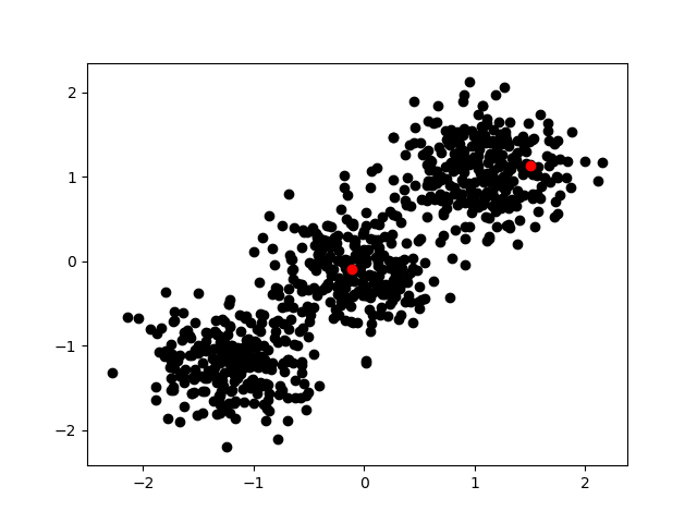
意図的にあからさまな３クラスタの分布を作成しクラスタ検出してみた
赤い点が本ロジックにより尤もクラスタ中心らしいとされたサンプルです

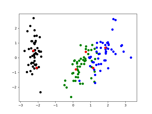
Irisデータセットに対して使ってみた
赤い点が本ロジックにより尤もクラスタ中心らしいとされたサンプルです

以下、手法について解説していきます

１つ目のクラスタを決定する

https://qiita.com/ikuo0/items/4ff7e1106e56b7b56b95
こちらを参照
密度係数の一番高いサンプルを１つ目のクラスタとします

２つ目以降のクラスタを決定していく

サンプルから既に発見されたクラスタまでの距離を算出、その中で一番小さい値を ”距離係数” とする
Ａ、Ｂ、Ｃ の３サンプルがあり、ＢとＣは検出済みのクラスタとして
Ａ → Ｂ の距離が１
Ａ → Ｃ の距離が３
だとするなら短い距離を採用しサンプルＡの距離係数は１となる

前項の
＞＞１つ目のクラスタを決定する
で算出した ”密度係数” と 距離係数 を掛けてその値を ”クラスタ係数” とする
クラスタ係数の一番大きなサンプルが次のクラスタとなる
これを任意の数だけ繰り返します。

この工程では最寄りのクラスタまでの距離ができるだけ遠いサンプル　かつ　密度係数の高いサンプル　を探しています

クラスタ検出の順序１

意図的に作ったあからさまな３クラスタについて６回のクラスタ検出を実施したプロットです

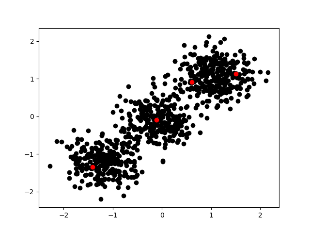
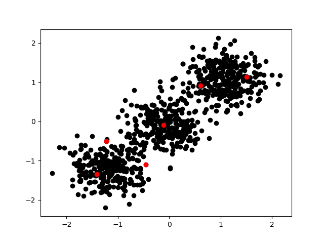
この時に密度係数は
[1. 0.62404961 0.60945085 0.6840667 0.36270498 0.42035119 0.34232924]
このようになっていました

クラスタ検出の順序２

Irisデータセットに対して６回のクラスタ検出を実施したプロットです
４次元データのままクラスタ検出を実施しプロットの際だけPCAで２次元圧縮した物を使用しています

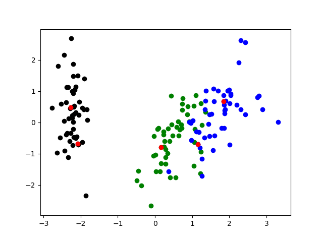
この時に密度係数は
[1. 0.47633577 0.35270676 0.37194045 0.36089639 0.3314366 0.3979942 ]
このようになっていました

密度係数を最適なクラスタ数の指標にする

変化が急な下降をした箇所、又は変化が平坦になり始めた箇所の前後が最適なクラスタ数かもしれないと考えられます

[1. 0.62404961 0.60945085 0.6840667 0.36270498 0.42035119 0.34232924]
このような変化であれば最適なクラスタ数は２個以上かなと考えられます

[1. 0.47633577 0.35270676 0.37194045 0.36089639 0.3314366 0.3979942 ]
このような変化であれば最適なクラスタ数は２個以上かなと考えられます

密度係数が上昇に転じている箇所は明らかにクラスタ数が多すぎると思って良いでしょう
ですので

[1. 0.62404961 0.60945085 0.6840667 0.36270498 0.42035119 0.34232924]
このような変化であればクラスタ数は多くても５個だと考えられます

[1. 0.47633577 0.35270676 0.37194045 0.36089639 0.3314366 0.3979942 ]
このような変化であればクラスタ数は多くても６個だと考えられます

検証不足について

検証不足のような感じはするんですが証明するための手法も思いつかないのでとりあえず今回はここまでとします
検証方法なり明らかな欠陥が思いついたら追加の記事を書きたいと思います

そもそもの話、クラスタ数がいくつなら良いか？という話は目的により異なると思っているのでなにをもって正しいというのか難しいです
解析がしたいのか、機械学習の特徴作りの過程として必要なのかとか、事情により正解は変わってくると思っています

実験に使ったソースコード

import matplotlib.pyplot as plot
import numpy as np
import random
import sklearn.datasets
import sklearn.decomposition
import sys

def standardziation(x):
    avr = np.mean(x, axis=0)
    std = np.std(x, axis=0)
    return (x - avr) / std

def normalization(x):
    xmin = np.min(x, axis=0)
    xmax = np.max(x, axis=0)
    return (x - xmin) / (xmax - xmin)

def densest(x, min_distance=1e-3):
    distances = []
    for i, ix in enumerate(x):
        d = 0
        for j, jx in enumerate(x):
            if j == i: continue
            id = np.linalg.norm(ix - jx)
            d += 1 / (id + 1e-2) # バラツキのあるクラスタ中心を出したいとき
            #d += 1 / (id + min_distance) # 密度の高いクラスタ中心を出したいとき
        distances.append(d)
    return np.array(distances)

def distance_samples(x, samples):
    distances = []
    for ix in x:
        darr = []
        for sample in samples:
            darr.append(np.linalg.norm((ix - sample) ** 2))
        distances.append(np.min(darr))
    distances = np.array(distances)
    return distances

def createDistribution1(counter):
    samples = []
    for cnt in counter:
        sample = []
        for i in range(cnt):
            sample.append(random.gauss(0,1))
        samples.append(sample)
    
    y = []
    for i in range(len(counter)):
        for j in range(len(samples[i])):
            y.append(samples[i][j] + i * 3)
    return np.array(y)

def createDistribution2(counter):
    xx, yy = [], []
    for cnt in counter:
        ix, iy = [], []
        for i in range(cnt):
            ix.append(random.gauss(0,1))
            iy.append(random.gauss(0,1))
        xx.append(ix)
        yy.append(iy)
    
    x, y = [], []
    for i in range(len(counter)):
        for j in range(len(xx[i])):
            x.append(xx[i][j] + i * 3)
            y.append(yy[i][j] + i * 3)
    return x, y

def clear_plot():
    plot.clf()

def Test1():
    clear_plot()
    x = [1, 11, 12, 13, 20]
    y = [0, 0, 0, 0, 0]
    
    nx = np.array(x).reshape(-1, 1)
    ny = np.array(y).reshape(-1, 1)
    nx = standardziation(nx)
    
    densest_coefficient = densest(nx)
    densest_coefficient = normalization(densest_coefficient)
    densest_idx = np.argmax(densest_coefficient)
    
    plot.scatter(x, y, c="black");
    plot.scatter([x[densest_idx]], [y[densest_idx]], c="red");
    plot.savefig("test1.png");

def Test2():
    clear_plot()
    x = [1, 11, 12, 13]
    y = [0, 0, 0, 0]
    
    nx = np.array(x).reshape(-1, 1)
    ny = np.array(y).reshape(-1)
    nx = standardziation(nx)
    
    densest_coefficient = densest(nx)
    densest_coefficient = normalization(densest_coefficient)
    densest_idx = np.argmax(densest_coefficient)
    
    plot.scatter(x, y, c="black");
    plot.scatter([x[densest_idx]], [y[densest_idx]], c="red");
    plot.savefig("test2.png");

def Test3():
    clear_plot()
    x = createDistribution1([200, 100, 300]);
    x = standardziation(x)
    y = np.zeros(len(x))
    
    nx = np.array(x).reshape(-1, 1)
    densest_coefficient = densest(nx)
    densest_coefficient = normalization(densest_coefficient)
    densest_idx = np.argmax(densest_coefficient)
    densest_idxs = [densest_idx]
    
    plot.hist(x, bins=100)
    plot.savefig("test3_hist.png");
    
    clear_plot()
    plot.scatter(x, y, c="black");
    plot.scatter([x[densest_idx]], [y[densest_idx]], c="red");
    for i in range(5):
        distances = distance_samples(nx, np.array(nx[densest_idxs]))
        distances = normalization(distances)
        coeff = distances * densest_coefficient
        next_densest_idx = np.argmax(coeff)
        densest_idxs.append(next_densest_idx)
        plot.scatter([x[next_densest_idx]], [y[next_densest_idx]], c="red");
        print("densest_idxs", densest_idxs)
    plot.savefig("test3_scatter.png");
    print(densest_coefficient[densest_idxs])

def Test4():
    clear_plot()
    #x, y = createDistribution2([200, 100, 300]);
    #x, y = createDistribution2([300, 300, 300]);
    #x, y = createDistribution2([300, 250, 250]);
    x, y = createDistribution2([250, 250, 300]);
    xy = np.c_[x, y]
    xy = standardziation(xy)
    
    densest_coefficient = densest(xy)
    densest_coefficient = normalization(densest_coefficient)
    densest_idx = np.argmax(densest_coefficient)
    densest_idxs = [densest_idx]
    
    
    plot.scatter(xy[:,0], xy[:,1], c="black")
    plot.scatter(xy[:,0][densest_idx], xy[:,1][densest_idx], c="red")
    for i in range(6):
        plot.savefig("test4_{:2}.png".format(i));
        distances = distance_samples(xy, np.array(xy[densest_idxs]))
        distances = normalization(distances)
        coeff = distances * densest_coefficient
        next_densest_idx = np.argmax(coeff)
        densest_idxs.append(next_densest_idx)
        plot.scatter([xy[:,0][next_densest_idx]], [xy[:,1][next_densest_idx]], c="red");
    print(densest_coefficient[densest_idxs])

def Test5():
    clear_plot()
    data = sklearn.datasets.load_iris()
    x = data["data"]
    x = standardziation(x)
    y = data["target"]
    setosa_idx = np.where(y == 0)[0]
    versicolor_idx = np.where(y == 1)[0]
    virginica_idx = np.where(y == 2)[0]
    
    densest_coefficient = densest(x)
    densest_coefficient = normalization(densest_coefficient)
    densest_idx = np.argmax(densest_coefficient)
    densest_idxs = [densest_idx]
    
    model = sklearn.decomposition.PCA(n_components=2)
    model.fit(x)
    X = model.transform(x)
    
    colors = ["black", "green", "blue"]
    for i, idxs in enumerate([setosa_idx, versicolor_idx, virginica_idx]):
        for idx in idxs:
            plot.scatter(X[:,0][idx], X[:,1][idx], c=colors[i])
    
    plot.scatter(X[:,0][densest_idx], X[:,1][densest_idx], c="red")
    for i in range(6):
        plot.savefig("test5_{:2}.png".format(i));
        distances = distance_samples(x, np.array(x[densest_idxs]))
        distances = normalization(distances)
        coeff = distances * densest_coefficient
        next_densest_idx = np.argmax(coeff)
        densest_idxs.append(next_densest_idx)
        plot.scatter([X[:,0][next_densest_idx]], [X[:,1][next_densest_idx]], c="red");
    
    print(densest_coefficient[densest_idxs])
    

if __name__ == "__main__":
    #Test1()
    #Test2()
    #Test3()
    Test4()
    Test5()