尤もクラスタらしいクラスタの中心を検出する

いくつかのクラスタがあるサンプル郡の中で密度が高いクラスタの概ね中心になるサンプルを検出します
本ロジックは KMEANS や GMM のようなEMアルゴリズムを使わず一定の計算数で検出したいという条件があります

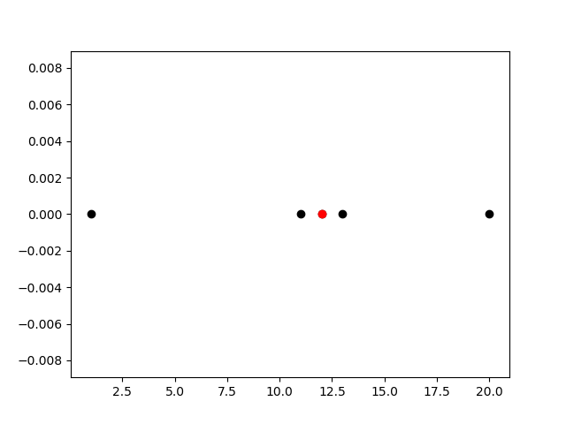
この画像の赤い点を見つけるロジックを考えます
このサンプルは左から250個のクラスタ、250個のクラスタ、300個のクラスタとなるよう意図的に作られたサンプルです

方法

全てのサンプルにおいて全てのサンプルからの距離の逆数の和を計算します
”全てのサンプルからの距離の逆数の和”　を”密度係数”とします
密度係数が最も大きい箇所を密度の高い場所とします

図のように一次元上に並んだサンプルの密度係数を計算してみます
Ａの密度係数を計算します
Bまでの距離 1（逆数は 1/1）
Cまでの距離 2^2（逆数は 1/4）
Dまでの距離 6^2（逆数は 1/36）
Ａの密係数＝1+(1/4)+(1/36)=1.277...

同様にＢ、Ｃ、Ｄの密度係数を計算します

Ｂの密度係数＝ (1/1^2)+(1/1^2)+(1/5^2) = 2.04
Ｃの密度係数＝ (1/2^2)+(1/1^1)+(1/4^2) = 1.3125
Ｄの密度係数＝ (1/6^2)+(1/5^2)+(1/4^2) = 0.13027...

Ａ＝ 1.277
Ｂ＝ 2.04
Ｃ＝ 1.312
Ｄ＝ 0.130

となり密度の一番高い箇所はＢということになり、なんらかのクラスタ中心である可能性が高いと言えます

実験結果

単純なサンプル１

単純なサンプル２

ランダムな一次元サンプルによる実験

ランダムな二次元サンプルによる実験

Irisデータセットによる実験

versicolor と virginica が近いため同一クラスタと認識した結果となっていますが、概ね群れの中心を指す場所を出せていると思います

実験結果を見ると問題無く動作しているように見えますがサンプル密度により意図しない動作をします
ソースコードの後に問題点を解説します

ソースコード

import matplotlib.pyplot as plot
import numpy as np
import random
import sklearn.datasets
import sklearn.decomposition
import sys

def standardziation(x):
    avr = np.mean(x, axis=0)
    std = np.std(x, axis=0)
    return (x - avr) / std

def densest_index1(x):
    distance = []
    for i, ix in enumerate(x):
        d = 0
        for j, jx in enumerate(x):
            d += np.linalg.norm(ix - jx)
        distance.append(d)
    return np.argmin(distance)

def densest_index2(x):
    distance = []
    for i, ix in enumerate(x):
        d = 0
        for j, jx in enumerate(x):
            if j == i: continue
            id = np.linalg.norm(ix - jx)
            #d += 1 / (id + 1e-2) # バラツキのあるクラスタ中心を出したい時
            d += 1 / (id + 1e-3) # 密度の高いクラスタ中心を出したい時
        distance.append(d)
    return np.argmax(distance)

def densest_index(x):
    #return densest_index1(x)
    return densest_index2(x)

def createDistribution1(counter):
    samples = []
    for cnt in counter:
        sample = []
        for i in range(cnt):
            sample.append(random.gauss(0,1))
        samples.append(sample)
    
    y = []
    for i in range(len(counter)):
        for j in range(len(samples[i])):
            y.append(samples[i][j] + i * 3)
    return np.array(y)

def createDistribution2(counter):
    xx, yy = [], []
    for cnt in counter:
        ix, iy = [], []
        for i in range(cnt):
            ix.append(random.gauss(0,1))
            iy.append(random.gauss(0,1))
        xx.append(ix)
        yy.append(iy)
    
    x, y = [], []
    for i in range(len(counter)):
        for j in range(len(xx[i])):
            x.append(xx[i][j] + i * 3)
            y.append(yy[i][j] + i * 3)
    return x, y

def clear_plot():
    plot.clf()

def Test1():
    clear_plot()
    x = [1, 11, 12, 13, 20]
    y = [0, 0, 0, 0, 0]
    
    nx = np.array(x).reshape(-1, 1)
    ny = np.array(y).reshape(-1)
    idx = densest_index(nx)
    
    plot.scatter(x, y, c="black");
    plot.scatter([x[idx]], [y[idx]], c="red");
    plot.savefig("test1.png");

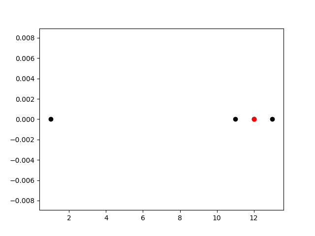
def Test2():
    clear_plot()
    x = [1, 11, 12, 13]
    y = [0, 0, 0, 0]
    
    nx = np.array(x).reshape(-1, 1)
    ny = np.array(y).reshape(-1)
    idx = densest_index(nx)
    
    plot.scatter(x, y, c="black");
    plot.scatter([x[idx]], [y[idx]], c="red");
    plot.savefig("test2.png");

def Test3():
    clear_plot()
    x = createDistribution1([200, 100, 300]);
    x = standardziation(x)
    y = np.zeros(len(x))
    idx = densest_index(np.array(x).reshape(-1, 1))
    
    plot.hist(x, bins=100)
    plot.savefig("test3_hist.png");
    
    clear_plot()
    plot.scatter(x, y, c="black");
    plot.scatter([x[idx]], [y[idx]], c="red");
    plot.savefig("test3_scatter.png");

def Test4():
    clear_plot()
    #x, y = createDistribution2([200, 100, 300]);
    #x, y = createDistribution2([300, 300, 300]);
    #x, y = createDistribution2([300, 250, 250]);
    x, y = createDistribution2([250, 250, 300]);
    xy = np.c_[x, y]
    xy = standardziation(xy)
    idx = densest_index(xy)
    plot.scatter(xy[:,0], xy[:,1], c="black")
    plot.scatter(xy[:,0][idx], xy[:,1][idx], c="red")
    plot.savefig("test4.png");

def Test5():
    clear_plot()
    data = sklearn.datasets.load_iris()
    x = data["data"]
    x = standardziation(x)
    y = data["target"]
    setosa_idx = np.where(y == 0)[0]
    versicolor_idx = np.where(y == 1)[0]
    virginica_idx = np.where(y == 2)[0]
    dense_idx = densest_index(x)
    model = sklearn.decomposition.PCA(n_components=2)
    model.fit(x)
    X = model.transform(x)
    
    colors = ["black", "green", "blue"]
    for i, idxs in enumerate([setosa_idx, versicolor_idx, virginica_idx]):
        for idx in idxs:
            plot.scatter(X[:,0][idx], X[:,1][idx], c=colors[i])
    
    plot.scatter(X[:,0][dense_idx], X[:,1][dense_idx], c="red")
    plot.savefig("test5.png");

if __name__ == "__main__":
    Test1()
    Test2()
    Test3()
    Test4()
    Test5()

# python main.py

問題点

            #d += 1 / (id + 1e-2) # バラツキのあるクラスタ中心を出したい時
            d += 1 / (id + 1e-3) # 密度の高いクラスタ中心を出したい時

ここが問題の箇所です
０割りの回避を行っている部分ですが、最小値（1e-2 とか 1e-3）の定義により一定以上の密度の高さを無視するようになります
極端な例ですが、全てのサンプルは１以上の距離があるという状態で１００個のクラスタと離れた場所にある１０個のクラスタがあったとします
１０個のクラスタのほうに 1e-100 しか距離の離れていないサンプルを１個だけ追加します
人間的な感覚では１００個のクラスタ中心を”最もクラスタらしいクラスタだ”と検出してほしいわけですが
1e-100 等とても小さい距離だけ離れているサンプルが１個でも存在していると密度係数は1e+100以上の値を出してしまい１０個の群れのほうをクラスタだと検出します

＞最小値（1e-2 とか 1e-3）の定義により一定以上の密度の高さを無視するようになります
人為的に最小値を設定しないと意図した通りに動かない事が問題点というか、注意すべき箇所となります
プロットの見た目の形状よりも”密度の高い点こそがクラスタである”　としたい場合は最小値定義を低く設定します（1e-3 等）
プロットの見た目の形状の通り”面積（体積？）の大きな塊こそがクラスタである”　としたい場合は最小値定義を大きく設定します（1e-2 等）
※サンプルは標準化されている事が前提です

一定以上の密度の無視＝広範囲の広がりも許容する　という調整ができると捉えればメリットなのかもしれません

既にありそうだなとも思いましたが検索しても出てこないので作りました
どういう単語で検索すればいいのかも分からなかったので似たような処理が既に存在するなら教えて頂けるとありがたいです
以上です