ハフ変換で直線を検出する実装

ハフ変換で直線を検出する

ハフ変換でどの辺に直線があるかを検出します。
厳密にどこからどこに直線があったかまでの検出は行わず描画範囲内のある距離・ある角度に直線が存在しているかの検出だけを行います、ハフ変換自体は解説が多いので解説はせず実装だけを乗せていきます。
実装する上で参考にしたサイトは下記です。
http://www.allisone.co.jp/html/Notes/image/Hough/index.html
https://jp.mathworks.com/discovery/image-transform.html
https://qiita.com/YSRKEN/items/ee94c7c22599c2374722
https://codezine.jp/article/detail/153
https://qiita.com/tifa2chan/items/d2b6c476d9f527785414

おおまかな手順

１．画像を２値化（白黒画像化）する
２．描画されている点全てにハフ変換を実行して角度と距離を算出する
３．Ｘ軸を距離、Ｙ軸を角度とした２次元配列で「２」のデータを２次元ヒストグラム（ヒートマップ）化する
４．「３」のデータの頂点（角度・距離が同一で数の多い点）の線が存在している可能性が分かる
５．「４」のデータ数の多い上位ｎ個を検出された線とする

手順「３～４」の２次元ヒストグラムの頂点検出はそのままでは困難であるためガウシアンフィルタで平滑化を行ってから行う、その際の誤検出については上位ｎ個というフィルタでだいたい弾かれるので問題無いというスタンスである

「３．Ｘ軸を距離、Ｙ軸を角度とした～」部分について本実装のプロットではX軸Y軸が逆になっているが、実データでは解説の通りである、ハフ変換プロットと向きを合わせるため解説に合わせずにそのままにしてある。

実装

以下実装となります、jupyterにコピペすれば動くはずです。
サンプル画像を作る所から実装してあります。

import inspect
import math
import matplotlib
import matplotlib.pyplot as plt
import numpy as np
import PIL.Image
import random
import scipy.ndimage

CANVAS_WIDTH = 300
CANVAS_HEIGHT = 200

def plotLine(dst, x1, y1, x2, y2, broken=1, variance=1):
    xd = x2 - x1
    yd = y2 - y1
    xsize = len(dst[0])
    ysize = len(dst)

    if xd == 0:
        if y1 > y2:
            y1, y2 = y2, y1
        for i in range(int(y1), int(y2), 1):
            dst[i][x1] = 1
        return

    if yd == 0:
        if x1 > x2:
            x1, x2 = x2, x1
        for i in range(int(x1), int(x2), 1):
            dst[y1][i] = 1
        return

    rad = math.atan2(yd, xd)
    distance = math.sqrt((xd ** 2) + (yd ** 2))
    for i in range(int(distance)):
        if broken >= 2 and not (i % broken) == 0: continue
        x = x1 + i * math.cos(rad)
        y = y1 + i * math.sin(rad)
        if variance > 0:
            x += int(random.random() * variance) - (variance / 2)
            y += int(random.random() * variance) - (variance / 2)
        if x < 0: x = 0
        if x >= xsize: x = xsize - 1
        if y < 0: y = 0
        if y >= ysize: y = ysize - 1
        dst[int(y)][int(x)] = 1

def createSampleImage(width, height):
    x = np.zeros((height, width)).astype(np.uint8)
    for i in range(4):
        x1 = int(random.uniform(0, CAMVAS_WIDTH))
        y1 = int(random.uniform(0, CAMVAS_HEIGHT))
        x2 = int(random.uniform(0, CAMVAS_WIDTH))
        y2 = int(random.uniform(0, CAMVAS_HEIGHT))
        plotLine(x, x1, y1, x2, y2, broken=0, variance=0)
    return x

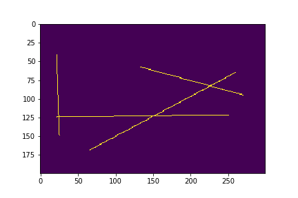
# 直線のサンプル画像を作成する
random.seed(63)
imageData = createSampleImage(CANVAS_WIDTH, CANVAS_HEIGHT)
plt.imshow(imageData)
plt.savefig("./002_sample_image.png")
plt.show()

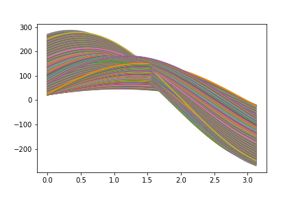
# ハフ変換
def houghConvertSub(theta, x, y):
    distance = []
    for t in theta:
        d = x * math.cos(t) + y * math.sin(t)
        distance.append(d)
    return distance

PY, PX = np.where(imageData == 1) # # ピクセル座標の取得
DegreeDiscrete = 180 # pi をいくつに分割するか（粒度をどの程度にするか）、100とか200でも良い
theta_arr = [math.pi * (i / DegreeDiscrete) for i in range(0, DegreeDiscrete)]
PR = []
for x, y in zip(PX, PY):
    p = houghConvertSub(theta_arr, x, y)
    PR.append(p)

PR = np.array(PR)
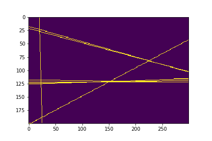
plt.plot(theta_arr, PR.transpose())
plt.savefig("./003_haough_convert.png")
plt.show()

print("len(PX)", len(PX))
print("len(PY)", len(PY))
print("len(theta_arr)", len(theta_arr))

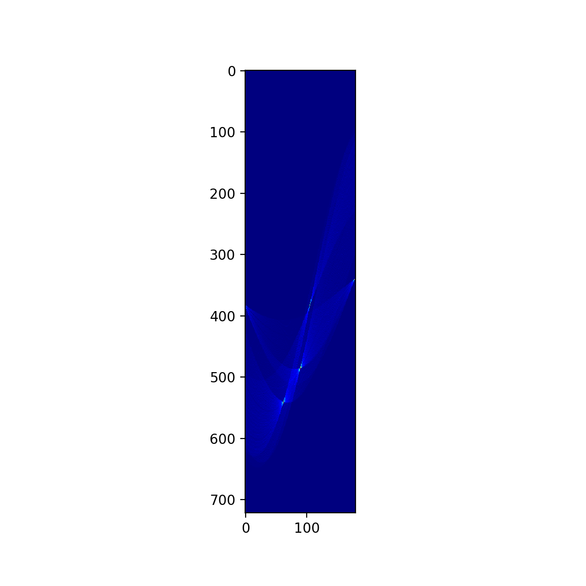
# 2次元配列にして交差している点をカウントする
# 対角線の長さを求め距離の最大値とする
diagonalDistance = math.sqrt((CANVAS_WIDTH ** 2) + (CANVAS_HEIGHT ** 2))
diagonalDistance = round(diagonalDistance)

# 交差点の交差数を投票する2次元配列を作成
vote = np.zeros((diagonalDistance * 2, len(theta_arr)))
print("ballot.shape", ballot.shape)
for P in PR:
    for x, p in enumerate(P):
        y = int(round(p))
        vote[y + diagonalDistance][x] += 1

# 標準化しておく
vote = (vote - np.mean(vote)) / np.std(vote)

plt.figure(figsize=(6,6),dpi=200)
plt.imshow(vote, cmap='jet', interpolation='nearest')
plt.savefig("./004_haough_convert_vote.png")
plt.show()

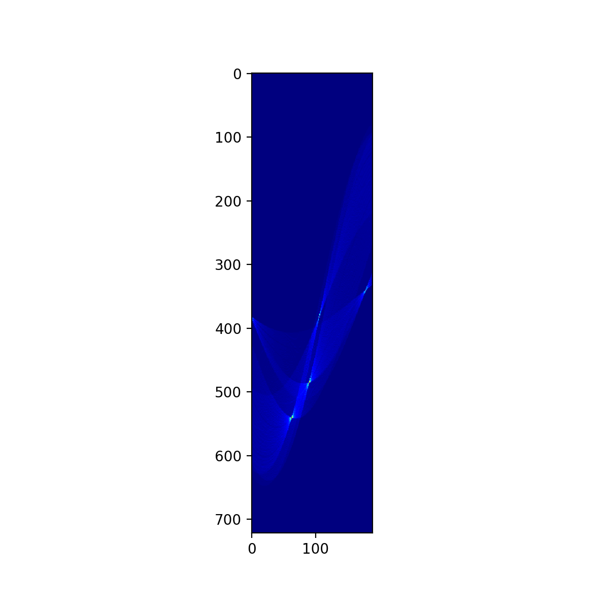
# 角度がループする都合上、先頭列と列の末尾はデータとしては連続している
# 列末尾に先頭列をいくつか追加しておく事で一括で処理できるよう準備する
appendMat = np.flipud(vote[:,:10])
newVote = np.c_[vote, appendMat]
print("newVote.shape", newVote.shape)

plt.figure(figsize=(6,6),dpi=200)
plt.imshow(newVote, cmap='jet', interpolation='nearest')
plt.savefig("./005_haough_convert_vote_ex.png")
plt.show()

# ガウシアンフィルタをかけて頂点をできるだけ検出しやすくする
filteredVote = scipy.ndimage.gaussian_filter(newVote, sigma=0.5)
plt.figure(figsize=(6,6),dpi=200)
plt.imshow(filteredVote, cmap='jet', interpolation='nearest')
plt.savefig("./006_haough_convert_vote_gaussian.png")
plt.show()

def detectPeak1D(x):
    conv1 = np.convolve(x, [1, -1], mode="full")
    flag1 = (conv1 > 0).astype(int)
    flag2 = (conv1 <= 0).astype(int)
    flag1 = flag1[:-1]
    flag2 = flag2[1:]
    flag3 = flag1 & flag2
    return flag3

def detectPeak2D(x):
    peaks1 = []
    for ix in x:
        peak = detectPeak1D(ix)
        peaks1.append(peak)
    peaks1 = np.array(peaks1)
    peaks2 = []
    for ix in x.transpose():
        peak = detectPeak1D(ix)
        peaks2.append(peak)
    peaks2 = np.array(peaks2).transpose()
    flag = (peaks1 & peaks2).astype(int)
    return flag

# ピーク検出を行う
# 誤検知については後の処理で投票数の少ない頂点を間引く事で対応する
peaks = detectPeak2D(filteredVote)
xidx, yidx = np.where(peaks == 1)
print("np.max(filteredVote)", np.max(filteredVote))
for x, y in zip(xidx, yidx):
    if filteredVote[x][y] > 10:
        peaks[x][y] = 1
    else:
        peaks[x][y] = 0

plt.figure(figsize=(8,8),dpi=200)
plt.imshow(peaks, cmap='spring', interpolation='nearest')
plt.savefig("./007_haough_convert_peaks.png")
plt.show()

# ピークからθのインデックスを取り出す
idxs = np.where(peaks != 0)
peakValues = filteredVote[idxs]

print(idxs[0])
print(idxs[1])
distances = idxs[0]
thetaIndexes  =[]
for idx in idxs[1]:
    if idx >= DegreeDiscrete:# 先頭末尾を繋げた部分について、インデックスを修正する
        idx = idx - DegreeDiscrete
    thetaIndexes.append(idx)

distances = np.array(distances)
thetaIndexes = np.array(thetaIndexes)

print(distances)
print(thetaIndexes)
print("len(PX)", len(PX))
print("len(PY)", len(PY))
print("len(PR)", len(PR))
print("len(THETA)", len(THETA))

# ピークの上位10個だけを採用する
idxs = np.argsort(peakValues)[::-1]
idxs = idxs[:10]
distances = distances[idxs]
thetaIndexes = thetaIndexes[idxs]

# 検出された直線を実際に描画して確認する
#y = -(math.cos(rad) / math.sin(rad)) * x + ((yidx[0] - diagonalDistance) / math.sin(rad))
#x = -(math.sin(rad) / math.cos(rad)) * y + ((yidx[0] - diagonalDistance) / math.cos(rad))
x = np.zeros((CANVAS_HEIGHT, CANVAS_WIDTH)).astype(np.uint8)

threshold1 = math.pi * (3/4)
threshold2 = math.pi * (1/4)
for idx, d in zip(thetaIndexes, distances):
    rad = theta_arr[idx]
    #x= -y sinθ/cosθ +ρ/ cosθ
    #x1 = 
    if rad > (threshold1) or rad < (threshold2):
        y1 = 0
        y2 = CANVAS_HEIGHT
        x1 = -(math.sin(rad) / math.cos(rad)) * y1 + ((d - diagonalDistance) / math.cos(rad))
        x2 = -(math.sin(rad) / math.cos(rad)) * y2 + ((d - diagonalDistance) / math.cos(rad))
    else:
        x1 = 0
        x2 = CANVAS_WIDTH
        y1 = -(math.cos(rad) / math.sin(rad)) * x1 + ((d - diagonalDistance) / math.sin(rad))
        y2 = -(math.cos(rad) / math.sin(rad)) * x2 + ((d - diagonalDistance) / math.sin(rad))
    print(rad, x1, x2, y1, y2)
    plotLine(x, int(x1), int(y1), int(x2), int(y2), broken=1, variance=0)
plt.imshow(x)
plt.savefig("./009_haough_convert_lines.png")
plt.show()

解説が足りないですが、興味ある方はソースコードとコメントを読んでみてください。
以上です。