AutoGluonの基本的なAutoMLを試してみる
AutoGluonは、Amazonが開発したオープンソースのAutoMLフレームワークです。今回、AutoGluonを利用して以下のタスクに関するAutoML機能を試してみました。
- 表形式データの分類
- 表形式データの回帰
- 時系列予測
- 画像分類
今回試した以外にも、AutoGluonは以下のように様々なタスクに対応しています。
表形式データに関するタスク
- 表形式データの分類
- 表形式データの回帰
時系列データに関するタスク
- 時系列予測
Multimodalデータに関するタスク
Hugging Faceのモデルリポジトリを利用して、多様なマルチモーダルデータのタスクに対応しています。以下は対応しているタスクの例です。
- マルチモーダル表形式データの分類・回帰
- 画像分類
- 物体検出
- テキスト分類
- テキスト生成
- 翻訳
- OCR
前提条件
- AutoGluon Version: 1.5.0
- Python Version: 3.12.12
表形式データの分類
有名な分類タスク用データセットであるIrisデータセットを使った例です。まずはデータセットを準備します。
from sklearn import datasets
from sklearn.model_selection import train_test_split
import pandas as pd

dataset = datasets.load_iris()

df = pd.DataFrame(data=dataset.data, columns=dataset.feature_names)
df["target"] = dataset.target

train_df, test_df = train_test_split(df, test_size=0.2, random_state=42)

display(train_df.head())
display(test_df.head())
以下のようなデータです。
| sepal length (cm) | sepal width (cm) | petal length (cm) | petal width (cm) | target | |
|---|---|---|---|---|---|
| 22 | 4.6 | 3.6 | 1.0 | 0.2 | 0 |
| 15 | 5.7 | 4.4 | 1.5 | 0.4 | 0 |
| 65 | 6.7 | 3.1 | 4.4 | 1.4 | 1 |
| 11 | 4.8 | 3.4 | 1.6 | 0.2 | 0 |
| 42 | 4.4 | 3.2 | 1.3 | 0.2 | 0 |
| sepal length (cm) | sepal width (cm) | petal length (cm) | petal width (cm) | target | |
|---|---|---|---|---|---|
| 73 | 6.1 | 2.8 | 4.7 | 1.2 | 1 |
| 18 | 5.7 | 3.8 | 1.7 | 0.3 | 0 |
| 118 | 7.7 | 2.6 | 6.9 | 2.3 | 2 |
| 78 | 6.0 | 2.9 | 4.5 | 1.5 | 1 |
| 76 | 6.8 | 2.8 | 4.8 | 1.4 | 1 |
AutoGluon用のデータセット形式に変換します。
from autogluon.tabular import TabularDataset, TabularPredictor

train_data = TabularDataset(train_df)
test_data = TabularDataset(test_df)
あとは表形式データ用のPredictor(TabularPredictor)を作成し、学習・推論するだけです。
predictor = TabularPredictor(label="target").fit(train_data)
predictions = predictor.predict(test_data)
AutoGluonはデータの内容から分類タスクであることを自動的に判定してくれます。
=================== System Info ===================
[省略]
===================================================
[省略]
Train Data Rows:    120
Train Data Columns: 4
Label Column:       target
AutoGluon infers your prediction problem is: 'multiclass' (because dtype of label-column == int, but few unique label-values observed).
	3 unique label values:  [np.int64(0), np.int64(1), np.int64(2)]
	If 'multiclass' is not the correct problem_type, please manually specify the problem_type parameter during Predictor init (You may specify problem_type as one of: ['binary', 'multiclass', 'regression', 'quantile'])
Problem Type:       multiclass # <- multiclassになっています。
Preprocessing data ...
[省略]
推論結果は以下のようになっています。
predictions[:5]
73     1
18     0
118    2
78     1
76     1
Name: target, dtype: int64
評価指標を確認することもできます。
ret = predictor.evaluate(test_data, detailed_report=True)

ret_df = pd.DataFrame(ret["classification_report"])
display(ret_df)
| 0 | 1 | 2 | accuracy | macro avg | weighted avg | |
|---|---|---|---|---|---|---|
| precision | 1.0 | 1.000000 | 0.916667 | 0.966667 | 0.972222 | 0.969444 |
| recall | 1.0 | 0.888889 | 1.000000 | 0.966667 | 0.962963 | 0.966667 |
| f1-score | 1.0 | 0.941176 | 0.956522 | 0.966667 | 0.965899 | 0.966411 |
| support | 10.0 | 9.000000 | 11.000000 | 0.966667 | 30.000000 | 30.000000 |
AutoGluonが試したモデル毎の評価指標も確認することが可能です。
predictor.leaderboard(test_data, extra_metrics=["f1_macro"])
| model | score_test | f1_macro | score_val | eval_metric | pred_time_test | pred_time_val | fit_time | pred_time_test_marginal | pred_time_val_marginal | fit_time_marginal | stack_level | can_infer | fit_order | |
|---|---|---|---|---|---|---|---|---|---|---|---|---|---|---|
| 0 | LightGBMXT | 1.000000 | 1.000000 | 1.000000 | accuracy | 0.000729 | 0.000401 | 0.482431 | 0.000729 | 0.000401 | 0.482431 | 1 | True | 2 |
| 1 | CatBoost | 1.000000 | 1.000000 | 1.000000 | accuracy | 0.001354 | 0.000837 | 0.234552 | 0.001354 | 0.000837 | 0.234552 | 1 | True | 6 |
| 2 | LightGBMLarge | 1.000000 | 1.000000 | 1.000000 | accuracy | 0.001811 | 0.000400 | 2.694018 | 0.001811 | 0.000400 | 2.694018 | 1 | True | 11 |
| 3 | NeuralNetTorch | 1.000000 | 1.000000 | 1.000000 | accuracy | 0.002747 | 0.001838 | 1.232548 | 0.002747 | 0.001838 | 1.232548 | 1 | True | 10 |
| 4 | ExtraTreesEntr | 1.000000 | 1.000000 | 0.958333 | accuracy | 0.017640 | 0.013169 | 0.199860 | 0.017640 | 0.013169 | 0.199860 | 1 | True | 8 |
| 5 | ExtraTreesGini | 1.000000 | 1.000000 | 0.958333 | accuracy | 0.028808 | 0.014351 | 0.206514 | 0.028808 | 0.014351 | 0.206514 | 1 | True | 7 |
| 6 | RandomForestGini | 1.000000 | 1.000000 | 0.958333 | accuracy | 0.029583 | 0.013446 | 0.292962 | 0.029583 | 0.013446 | 0.292962 | 1 | True | 4 |
| 7 | RandomForestEntr | 1.000000 | 1.000000 | 0.958333 | accuracy | 0.030591 | 0.012489 | 0.197481 | 0.030591 | 0.012489 | 0.197481 | 1 | True | 5 |
| 8 | LightGBM | 0.966667 | 0.966583 | 1.000000 | accuracy | 0.001737 | 0.000393 | 0.899142 | 0.001737 | 0.000393 | 0.899142 | 1 | True | 3 |
| 9 | XGBoost | 0.966667 | 0.965899 | 0.916667 | accuracy | 0.005900 | 0.001184 | 0.556606 | 0.005900 | 0.001184 | 0.556606 | 1 | True | 9 |
| 10 | NeuralNetFastAI | 0.966667 | 0.965899 | 1.000000 | accuracy | 0.006194 | 0.004473 | 1.127240 | 0.006194 | 0.004473 | 1.127240 | 1 | True | 1 |
| 11 | WeightedEnsemble_L2 | 0.966667 | 0.965899 | 1.000000 | accuracy | 0.007086 | 0.004794 | 1.157533 | 0.000892 | 0.000321 | 0.030293 | 2 | True | 12 |
表形式データの回帰
回帰タスクのデータセットであるThe California housing datasetを利用した例です。まずはデータセットを準備します。
dataset = datasets.fetch_california_housing()

df = pd.DataFrame(data=dataset.data, columns=dataset.feature_names)
df["target"] = dataset.target

train_df, test_df = train_test_split(df[:1000], test_size=0.2, random_state=42)

display(train_df.head())
display(test_df.head())
| MedInc | HouseAge | AveRooms | AveBedrms | Population | AveOccup | Latitude | Longitude | target | |
|---|---|---|---|---|---|---|---|---|---|
| 29 | 1.6875 | 52.0 | 4.703226 | 1.032258 | 395.0 | 2.548387 | 37.84 | -122.28 | 1.320 |
| 535 | 5.2601 | 13.0 | 4.156379 | 1.100823 | 959.0 | 1.973251 | 37.78 | -122.27 | 2.927 |
| 695 | 2.4206 | 19.0 | 3.719613 | 1.089779 | 1765.0 | 2.437845 | 37.70 | -122.11 | 1.375 |
| 557 | 5.1039 | 52.0 | 5.628037 | 1.013084 | 1303.0 | 2.435514 | 37.76 | -122.23 | 2.738 |
| 836 | 4.3875 | 17.0 | 5.504983 | 1.059801 | 1873.0 | 3.111296 | 37.60 | -122.04 | 2.385 |
| MedInc | HouseAge | AveRooms | AveBedrms | Population | AveOccup | Latitude | Longitude | target | |
|---|---|---|---|---|---|---|---|---|---|
| 521 | 4.7188 | 52.0 | 7.068536 | 1.006231 | 805.0 | 2.507788 | 37.76 | -122.23 | 3.353 |
| 737 | 3.1734 | 38.0 | 6.060241 | 1.045181 | 880.0 | 2.650602 | 37.67 | -122.13 | 1.816 |
| 740 | 3.8676 | 40.0 | 5.514196 | 1.003155 | 914.0 | 2.883281 | 37.67 | -122.13 | 1.840 |
| 660 | 3.5547 | 36.0 | 5.609195 | 0.934866 | 672.0 | 2.574713 | 37.70 | -122.15 | 1.947 |
| 411 | 5.7912 | 52.0 | 7.291667 | 1.005952 | 412.0 | 2.452381 | 37.89 | -122.28 | 3.271 |
分類タスクと同様にAutoGluon用のデータセット形式に変換します。
train_data = TabularDataset(train_df)
test_data = TabularDataset(test_df)
学習・推論も分類タスクと同様です。AutoGluonが自動的にタスクの種類を判定してくれます。
predictor = TabularPredictor(label="target").fit(train_data)
predictions = predictor.predict(test_data)
=================== System Info ===================
[省略]
===================================================
[省略]
Train Data Rows:    800
Train Data Columns: 8
Label Column:       target
AutoGluon infers your prediction problem is: 'regression' (because dtype of label-column == float and many unique label-values observed).
	Label info (max, min, mean, stddev): (5.00001, 0.675, 2.12968, 0.89625)
	If 'regression' is not the correct problem_type, please manually specify the problem_type parameter during Predictor init (You may specify problem_type as one of: ['binary', 'multiclass', 'regression', 'quantile'])
Problem Type:       regression # <- regressionになっています。
Preprocessing data ...
[省略]
評価指標の出力も同様です。 root_mean_squared_error などが負数になっておりびっくりしますが、AutoGluonが符号を反転させているためです(評価指標が最大のモデルを選択するという比較方法で単純化しているらしい)。
ret = predictor.evaluate(test_data, detailed_report=True)

ret_df = pd.DataFrame([ret])
display(ret_df)
| root_mean_squared_error | mean_squared_error | mean_absolute_error | r2 | pearsonr | median_absolute_error | |
|---|---|---|---|---|---|---|
| 0 | -0.337892 | -0.114171 | -0.243167 | 0.842975 | 0.926857 | -0.168862 |
AutoGluonが評価したモデルも確認ができます。
predictor.leaderboard(test_data, extra_metrics=["r2"])
| model | score_test | r2 | score_val | eval_metric | pred_time_test | pred_time_val | fit_time | pred_time_test_marginal | pred_time_val_marginal | fit_time_marginal | stack_level | can_infer | fit_order | |
|---|---|---|---|---|---|---|---|---|---|---|---|---|---|---|
| 0 | LightGBMXT | -0.329303 | 0.850857 | -0.356802 | root_mean_squared_error | 0.006622 | 0.001256 | 2.019685 | 0.006622 | 0.001256 | 2.019685 | 1 | True | 1 |
| 1 | NeuralNetTorch | -0.331640 | 0.848732 | -0.436263 | root_mean_squared_error | 0.004493 | 0.003548 | 3.953525 | 0.004493 | 0.003548 | 3.953525 | 1 | True | 8 |
| 2 | CatBoost | -0.333273 | 0.847239 | -0.351505 | root_mean_squared_error | 0.001937 | 0.000442 | 0.245677 | 0.001937 | 0.000442 | 0.245677 | 1 | True | 4 |
| 3 | WeightedEnsemble_L2 | -0.337892 | 0.842975 | -0.334350 | root_mean_squared_error | 0.078949 | 0.057096 | 6.653374 | 0.001518 | 0.000184 | 0.004776 | 2 | True | 10 |
| 4 | RandomForestMSE | -0.346399 | 0.834968 | -0.353917 | root_mean_squared_error | 0.032986 | 0.025742 | 0.220570 | 0.032986 | 0.025742 | 0.220570 | 1 | True | 3 |
| 5 | ExtraTreesMSE | -0.346958 | 0.834435 | -0.344967 | root_mean_squared_error | 0.033604 | 0.025847 | 0.206870 | 0.033604 | 0.025847 | 0.206870 | 1 | True | 5 |
| 6 | LightGBM | -0.351175 | 0.830387 | -0.347429 | root_mean_squared_error | 0.001786 | 0.000523 | 1.538106 | 0.001786 | 0.000523 | 1.538106 | 1 | True | 2 |
| 7 | NeuralNetFastAI | -0.358509 | 0.823228 | -0.429565 | root_mean_squared_error | 0.006463 | 0.003125 | 0.405156 | 0.006463 | 0.003125 | 0.405156 | 1 | True | 6 |
| 8 | XGBoost | -0.360608 | 0.821153 | -0.352713 | root_mean_squared_error | 0.004562 | 0.001252 | 0.729527 | 0.004562 | 0.001252 | 0.729527 | 1 | True | 7 |
| 9 | LightGBMLarge | -0.380407 | 0.800974 | -0.365170 | root_mean_squared_error | 0.003996 | 0.000846 | 7.603294 | 0.003996 | 0.000846 | 7.603294 | 1 | True | 9 |
時系列予測
時系列予測では、Bike Sharing Demandデータセットを利用します。これは自転車シェアリングに関する需要の数を予測するものです。sklearnでもOpenML経由でデータセットの取得が可能ですが、そちらのバージョンは日付(datetime)の列がないため、今回はKaggleからダウンロードしたバージョンを利用しています。
# OpenMLから取得したデータセットだとdatetimeがないため、Kaggleのデータセットを使用します。事前にダウンロードが必要です。

df = pd.read_csv("data/bike-sharing-demand/train.csv", parse_dates=["datetime"])

df["item_id"] = 1  # 単一の時系列データとして扱うためのID列を追加

train_df = df[(df["datetime"] >= "2011-01-01") & (df["datetime"] <= "2012-09-30")]
test_df = df[(df["datetime"] >= "2012-10-01") & (df["datetime"] <= "2012-12-31")]

display(train_df.head())
display(test_df.head())
| datetime | season | holiday | workingday | weather | temp | atemp | humidity | windspeed | casual | registered | count | item_id | |
|---|---|---|---|---|---|---|---|---|---|---|---|---|---|
| 0 | 2011-01-01 00:00:00 | 1 | 0 | 0 | 1 | 9.84 | 14.395 | 81 | 0.0 | 3 | 13 | 16 | 1 |
| 1 | 2011-01-01 01:00:00 | 1 | 0 | 0 | 1 | 9.02 | 13.635 | 80 | 0.0 | 8 | 32 | 40 | 1 |
| 2 | 2011-01-01 02:00:00 | 1 | 0 | 0 | 1 | 9.02 | 13.635 | 80 | 0.0 | 5 | 27 | 32 | 1 |
| 3 | 2011-01-01 03:00:00 | 1 | 0 | 0 | 1 | 9.84 | 14.395 | 75 | 0.0 | 3 | 10 | 13 | 1 |
| 4 | 2011-01-01 04:00:00 | 1 | 0 | 0 | 1 | 9.84 | 14.395 | 75 | 0.0 | 0 | 1 | 1 | 1 |
| datetime | season | holiday | workingday | weather | temp | atemp | humidity | windspeed | casual | registered | count | item_id | |
|---|---|---|---|---|---|---|---|---|---|---|---|---|---|
| 9519 | 2012-10-01 00:00:00 | 4 | 0 | 1 | 1 | 18.86 | 22.725 | 72 | 7.0015 | 6 | 39 | 45 | 1 |
| 9520 | 2012-10-01 01:00:00 | 4 | 0 | 1 | 1 | 18.04 | 21.970 | 77 | 6.0032 | 5 | 13 | 18 | 1 |
| 9521 | 2012-10-01 02:00:00 | 4 | 0 | 1 | 1 | 18.86 | 22.725 | 72 | 0.0000 | 6 | 6 | 12 | 1 |
| 9522 | 2012-10-01 03:00:00 | 4 | 0 | 1 | 1 | 18.04 | 21.970 | 77 | 0.0000 | 1 | 6 | 7 | 1 |
| 9523 | 2012-10-01 04:00:00 | 4 | 0 | 1 | 1 | 17.22 | 21.210 | 82 | 7.0015 | 0 | 10 | 10 | 1 |
時系列予測でもAutoGluon用のデータセットに変換します。時系列予測専用のDataFrame(TimeSeriesDataFrame)になっている点に注意してください。
from autogluon.timeseries import TimeSeriesDataFrame, TimeSeriesPredictor

train_data = TimeSeriesDataFrame.from_data_frame(
    train_df, id_column="item_id", timestamp_column="datetime"
)
test_data = TimeSeriesDataFrame.from_data_frame(
    test_df, id_column="item_id", timestamp_column="datetime"
)

display(train_data.head())
display(test_data.head())
データセットを用意したら、時系列予測用のPredictor(TimeSeriesPredictor)を作成して学習を実行します。
predictor = TimeSeriesPredictor(
    prediction_length=48,
    freq="H",
    target="count",
    eval_metric="MASE",
)
predictor.fit(
    train_data,
    presets="medium_quality",
    time_limit=60,
)
以下は推論の例です。時系列予測は自己回帰であるため、予測の元となる部分を入力した上で、残りを推論する形になります。推論する部分を backtest_window として指定しています。
backtest_window = 100

predictions = predictor.predict(test_data[:-backtest_window])

display(predictions.head())
display(predictions.tail())
| mean | 0.1 | 0.2 | 0.3 | 0.4 | 0.5 | 0.6 | 0.7 | 0.8 | 0.9 | |
|---|---|---|---|---|---|---|---|---|---|---|
| item_id | timestamp | |||||||||
| 1 | 2012-12-15 20:00:00 | 194.065120 | 153.445508 | 165.888456 | 175.456589 | 185.240948 | 194.065120 | 202.139917 | 210.918463 | 220.560174 |
| 2012-12-15 21:00:00 | 174.495215 | 130.972268 | 145.480966 | 156.113247 | 165.878517 | 174.495215 | 183.074575 | 192.663728 | 203.698353 | |
| 2012-12-15 22:00:00 | 155.703548 | 117.243307 | 130.646849 | 140.136719 | 148.045559 | 155.703548 | 163.457911 | 171.482626 | 181.781609 | |
| 2012-12-15 23:00:00 | 137.703546 | 95.020458 | 109.967144 | 120.957801 | 129.799906 | 137.703546 | 145.535706 | 154.349331 | 165.599227 | |
| 2012-12-16 00:00:00 | 112.233787 | 75.123124 | 88.284815 | 97.711033 | 105.520264 | 112.233787 | 119.398298 | 127.307092 | 135.456921 |
| mean | 0.1 | 0.2 | 0.3 | 0.4 | 0.5 | 0.6 | 0.7 | 0.8 | 0.9 | |
|---|---|---|---|---|---|---|---|---|---|---|
| item_id | timestamp | |||||||||
| 1 | 2012-12-17 15:00:00 | 286.048873 | 196.198442 | 228.401797 | 251.165732 | 269.868576 | 286.048873 | 301.132948 | 315.901160 | 334.965616 |
| 2012-12-17 16:00:00 | 379.158938 | 274.415746 | 313.551948 | 338.641825 | 359.865772 | 379.158938 | 398.587786 | 417.644985 | 440.899046 | |
| 2012-12-17 17:00:00 | 578.996250 | 427.610388 | 499.315132 | 534.814860 | 558.817005 | 578.996250 | 601.253924 | 623.820675 | 654.386870 | |
| 2012-12-17 18:00:00 | 528.754239 | 395.574310 | 451.191804 | 484.078831 | 508.256391 | 528.754239 | 552.172252 | 574.361318 | 602.422813 | |
| 2012-12-17 19:00:00 | 369.496570 | 251.439543 | 296.232444 | 324.540943 | 348.070681 | 369.496570 | 390.179051 | 411.243000 | 436.956436 |
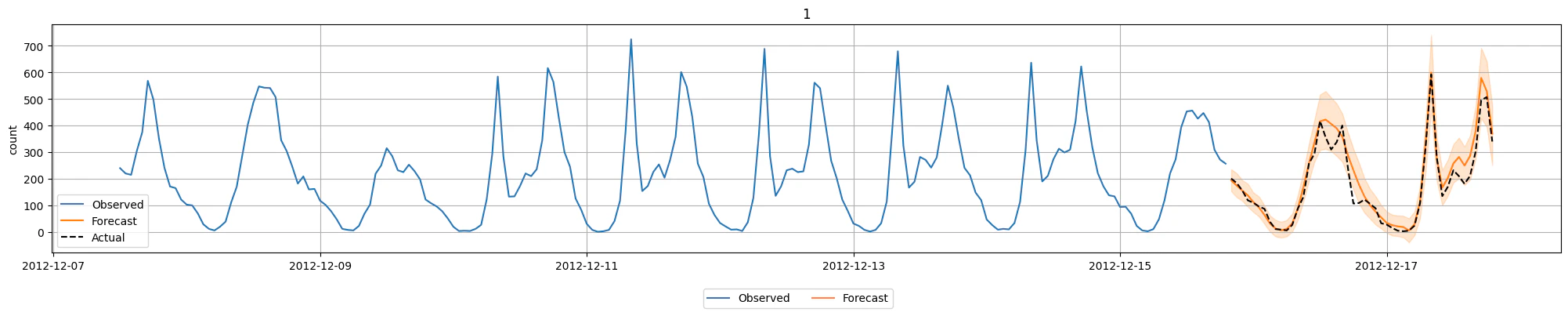
Predictorのplotで単純に結果を折れ線グラフで表示することもできますが、今回は推論部分の実績値も表示したいため、少し調整しています。
history_length = 200
fig = predictor.plot(
    test_data[:-backtest_window],
    predictions,
    quantile_levels=[0.1, 0.9],
    max_history_length=history_length,
)
ax = fig.axes[0] if hasattr(fig, "axes") and fig.axes else fig
item_id = test_data.item_ids[0]
actual_series = test_data.loc[item_id]["count"]
actual_series = actual_series[len(actual_series) - (history_length + backtest_window):]
actual_series = actual_series.reindex(predictions.index.get_level_values("timestamp"))
ax.plot(
    actual_series.index,
    actual_series.values,
    linestyle="--",
    color="black",
    label="Actual",
)
ax.legend()

fig
時系列予測でもAutoGluonが複数のモデルを評価します。leaderboardで評価内容を確認することができます。評価指標をMASEにしているのに負数になっているのは、前述のとおりAutoGluonが符号を判定しているためだと思われます。
predictor.leaderboard(test_data)
| model | score_test | score_val | pred_time_test | pred_time_val | fit_time_marginal | fit_order | |
|---|---|---|---|---|---|---|---|
| 0 | Chronos2 | -0.254466 | -1.184548 | 0.984460 | 0.594089 | 2.414695 | 5 |
| 1 | WeightedEnsemble | -0.262974 | -1.179862 | 2.248962 | 1.886012 | 0.093204 | 7 |
| 2 | DirectTabular | -0.341152 | -1.396010 | 0.032112 | 0.082884 | 3.028223 | 3 |
| 3 | SeasonalNaive | -0.435779 | -1.334797 | 1.263871 | 1.290907 | 0.010896 | 1 |
| 4 | RecursiveTabular | -0.517793 | -1.418418 | 0.079369 | 0.079426 | 4.486879 | 2 |
| 5 | TemporalFusionTransformer | -0.614487 | -1.521826 | 0.038884 | 0.020077 | 18.891045 | 6 |
| 6 | ETS | -0.925439 | -1.776815 | 3.892389 | 5.950521 | 0.012492 | 4 |
画像分類
AutoGluonではMultimodalデータに関するタスクとして、Hugging Faceのモデルリポジトリのモデルを利用して様々なタスクを実行することができます。今回はMNISTを利用した画像分類を試してみました。
以下はデータセットの準備処理です。画像をファイルに保存した上で、image(画像のファイルパス)/labelの列をもったDataFrameを用意します。なお、画像の前処理として0-255の範囲に正規化する処理を行っています。0-1ではない理由は、画像ファイルを人が見てわかりやすくするためです。
from PIL import Image
from autogluon.multimodal.utils import download
import os

dataset = datasets.load_digits()

train_data_size = 100
test_data_size = 10
train_images = dataset.images[:train_data_size].astype("uint8")
for i in range(train_images.shape[0]):
    train_images[i] = (train_images[i] / train_images[i].max()) * 255
train_labels = dataset.target[:train_data_size]
test_images = dataset.images[train_data_size : train_data_size + test_data_size].astype(
    "uint8"
)
for i in range(test_images.shape[0]):
    test_images[i] = (test_images[i] / test_images[i].max()) * 255
test_labels = dataset.target[train_data_size : train_data_size + test_data_size]

os.makedirs("tmp/train", exist_ok=True)
os.makedirs("tmp/test", exist_ok=True)

train_data = []
for i in range(len(train_images)):
    Image.fromarray(train_images[i]).save(f"tmp/train/digit_train_{i}.png")
    train_data.append(
        {
            "image": f"tmp/train/digit_train_{i}.png",
            "label": int(train_labels[i]),
        }
    )
test_data = []
for i in range(len(test_images)):
    Image.fromarray(test_images[i]).save(f"tmp/test/digit_test_{i}.png")
    test_data.append(
        {
            "image": f"tmp/test/digit_test_{i}.png",
            "label": int(test_labels[i]),
        }
    )

import matplotlib.pyplot as plt

fig, axes = plt.subplots(1, 10, figsize=(8, 8))
for i, ax in enumerate(axes.flat):
    ax.imshow(train_images[i], cmap="gray")
    ax.axis("off")
plt.show()

train_df = pd.DataFrame(train_data)
test_df = pd.DataFrame(test_data)

display(train_df.head())
display(test_df.head())

| image | label | |
|---|---|---|
| 0 | tmp/train/digit_train_0.png | 0 |
| 1 | tmp/train/digit_train_1.png | 1 |
| 2 | tmp/train/digit_train_2.png | 2 |
| 3 | tmp/train/digit_train_3.png | 3 |
| 4 | tmp/train/digit_train_4.png | 4 |
| image | label | |
|---|---|---|
| 0 | tmp/test/digit_test_0.png | 4 |
| 1 | tmp/test/digit_test_1.png | 0 |
| 2 | tmp/test/digit_test_2.png | 5 |
| 3 | tmp/test/digit_test_3.png | 3 |
| 4 | tmp/test/digit_test_4.png | 6 |
MultiModalPredictorを作成して学習を実行します。MultiModalPredictorもデータセットの内容から自動的にタスクの種類を判定し、必要なモデルをHugging Faceから自動的にダウンロードしてくれます。
from autogluon.multimodal import MultiModalPredictor
import uuid

model_path = f"./tmp/{uuid.uuid4().hex}-automm_mnist"
predictor = MultiModalPredictor(label="label", path=model_path)
predictor.fit(
    train_data=train_df,
    time_limit=120, # seconds
)
=================== System Info ===================
[省略]
===================================================
AutoGluon infers your prediction problem is: 'multiclass' (because dtype of label-column == int, but few unique label-values observed).
	10 unique label values:  [np.int64(0), np.int64(1), np.int64(2), np.int64(3), np.int64(4), np.int64(5), np.int64(6), np.int64(7), np.int64(8), np.int64(9)]
	If 'multiclass' is not the correct problem_type, please manually specify the problem_type parameter during Predictor init (You may specify problem_type as one of: ['binary', 'multiclass', 'regression', 'quantile'])

AutoMM starts to create your model. ✨✨✨
[省略]
INFO:timm.models._builder:Loading pretrained weights from Hugging Face hub (timm/caformer_b36.sail_in22k_ft_in1k)
INFO:timm.models._hub:[timm/caformer_b36.sail_in22k_ft_in1k] Safe alternative available for 'pytorch_model.bin' (as 'model.safetensors'). Loading weights using safetensors.
INFO:timm.models._builder:Missing keys (head.fc.fc2.weight, head.fc.fc2.bias) discovered while loading pretrained weights. This is expected if model is being adapted.
[省略]
今回選択された事前学習モデルは以下でした。
推論結果は以下の様に確認できます。
probs = predictor.predict_proba(
    {"image": [image_path for image_path in test_df["image"].tolist()]}
)

pd.DataFrame(
    {
        "pred": probs.argmax(axis=1),
        "prob": probs.max(axis=1),
        "actual": test_df["label"].tolist(),
    }
)
| pred | prob | actual | |
|---|---|---|---|
| 0 | 4 | 0.448798 | 4 |
| 1 | 0 | 0.869716 | 0 |
| 2 | 3 | 0.407478 | 5 |
| 3 | 3 | 0.650282 | 3 |
| 4 | 6 | 0.818564 | 6 |
| 5 | 9 | 0.253878 | 9 |
| 6 | 6 | 0.712888 | 6 |
| 7 | 1 | 0.872671 | 1 |
| 8 | 7 | 0.524540 | 7 |
| 9 | 3 | 0.411690 | 5 |
評価指標の確認は以下のとおりです。微妙な精度ですが、まずは動作確認まで。
scores = predictor.evaluate(test_df, metrics=["accuracy"])
print("Top-1 test acc: %.3f" % scores["accuracy"])
Top-1 test acc: 0.800