ディープラーニングの実装と過学習対策

はじめに

今回はディープラーニングの実装と過学習対策の実装です。
※初学者向けの内容となっています。

ディープラーニング概要

ディープラーニングとは、簡単に言うと「人間の脳の神経回路をマネして作ったニューラルネットワークをより複雑にしたもの」です。

🌟詳細はこちらの記事を参照してください。（ディープラーニングについてまとめました。）
https://qiita.com/hara_tatsu/items/c0e59b388823769f9704

🌟「畳み込みニューラルネットワーク（CNN）まとめ」
https://qiita.com/hara_tatsu/items/8dcd0a339ad2f67932e7

🌟畳み込みニューラルネットワーク（CNN）の実装
https://qiita.com/hara_tatsu/items/d2c6536ae35cca5e97ab

実装

今回は題材として、「【SIGNATE】国勢調査からの収入予測」を使います。
https://signate.jp/competitions/107

教育年数や職業等の国勢調査データから年収が$50,000ドルを超えるかどうかを予測するものです。

データの前処理

データの読み込みと整理

文字列データでは学習できないので、数値データに変換します。

python.py

import pandas as pd
import numpy as np

# データの読み込みと前処理
df = pd.read_csv('train.tsv', delimiter = '\t')
drop_list = ['id', 'occupation', 'native-country']
df = df.drop(drop_list, axis = 1)

#職業クラス
df= df.replace({'workclass':['?', 'Never-worked', 'Private', 'Without-pay']}, 0)
df= df.replace({'workclass':['Federal-gov', 'Local-gov', 'Self-emp-not-inc', 'State-gov']}, 1)
df= df.replace({'workclass':['Self-emp-inc']}, 2)
work = pd.crosstab(df['workclass'], df['Y'])

#教育
df = df.replace({'education': ['10th', '11th', '12th', '1st-4th', '5th-6th', '7th-8th', '9th', 'HS-grad', 'Preschool']}, 0)
df = df.replace({'education': ['Assoc-acdm', 'Assoc-voc', 'Bachelors', 'Prof-school', 'Some-college']}, 1)
df = df.replace({'education': ['Doctorate', 'Masters', 'Prof-school']}, 2)
edu = pd.crosstab(df['education'], df['Y'])

# 配偶者の有無
df = df.replace({'marital-status': ['Divorced', 'Married-spouse-absent', 'Never-married', 'Separated', 'Widowed']},0)
df = df.replace({'marital-status': ['Married-AF-spouse', 'Married-civ-spouse']}, 1)
mari = pd.crosstab(df['marital-status'], df['Y'])

# 関係
df = df.replace({'relationship': ['Not-in-family', 'Other-relative', 'Own-child', 'Unmarried']}, 0)
df = df.replace({'relationship': ['Husband', 'Wife']}, 1)
rela = pd.crosstab(df['relationship'], df['Y'])

# 人種
df = df.replace({'race': ['Amer-Indian-Eskimo', 'Black', 'Other']}, 0)
df = df.replace({'race': ['Asian-Pac-Islander', 'White']}, 1)
race = pd.crosstab(df['race'], df['Y'])

# 性別
df['sex'] = df['sex'].replace('Female', 0).replace('Male', 1) 
pd.crosstab(df['sex'], df['Y'])

#目的変数
df = df.replace({'Y': {'<=50K': 0, '>50K': 1}})

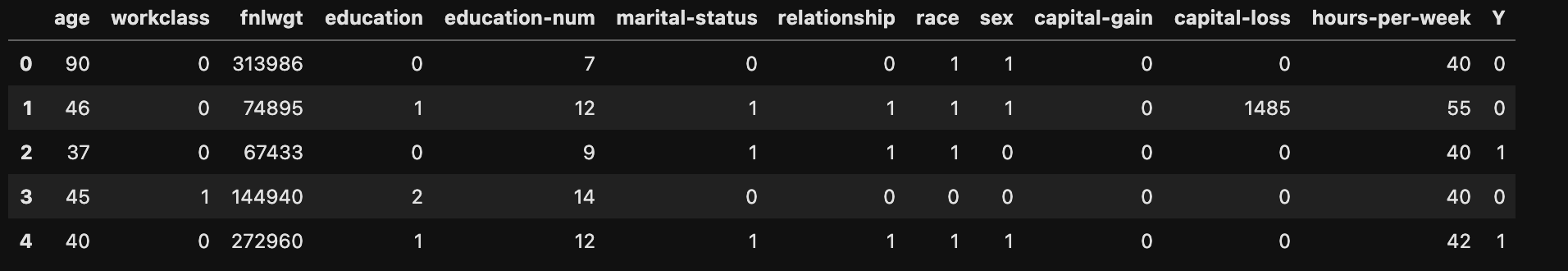
df.head()

処理後の結果。

説明変数と目的変数に分けてnumpy型に変換

python.py

#説明変数と目的変数に分ける
train = df.drop('Y', axis=1)
test = df['Y']

# numpy型に変換
train = train.values
test = test.values

print(train.shape)
print(train[:5])
print(test.shape)
print(test[:5])

(16280, 12)
[[    90      0 313986      0      7      0      0      1      1      0
       0     40]
 [    46      0  74895      1     12      1      1      1      1      0
    1485     55]
 [    37      0  67433      0      9      1      1      1      0      0
       0     40]
 [    45      1 144940      2     14      0      0      0      0      0
       0     40]
 [    40      0 272960      1     12      1      1      1      1      0
       0     42]]
(16280,)
[0 0 1 0 1]

データの標準化

データを見てわかるとおり、
①数値の幅が大きいデータがある
②データ間の数値の差が大きい
という状態です。

この状態だとディープラーニングはうまく学習することができません。

［-1, 1］又は［0, 1］の範囲の小さな値にスケーリングすることが必要になります。

python.py

from sklearn.preprocessing import StandardScaler

sc = StandardScaler()
#説明変数のみ標準化
train_std = sc.fit_transform(train)
train_std


array([[ 3.75931726, -0.54216861,  1.18232597, ..., -0.14742342,
        -0.21734177, -0.03330363],
       [ 0.54098621, -0.54216861, -1.09718324, ..., -0.14742342,
         3.44716207,  1.18508543],
       [-0.11730878, -0.54216861, -1.16832644, ..., -0.14742342,
        -0.21734177, -0.03330363],
       ...,
       [ 0.24841066, -0.54216861, -0.45335735, ..., -0.14742342,
        -0.21734177, -0.03330363],
       [-1.43389875, -0.54216861, -0.67445232, ..., -0.14742342,
        -0.21734177, -2.06395207],
       [-0.77560377, -0.54216861,  1.08401068, ...,  0.25702536,
        -0.21734177, -1.65782238]])

全ての数値を［-1, 1］の間の数値に変換しました。

訓練データ・評価データ・テストデータに分ける

python.py

from sklearn.model_selection import train_test_split

X_train, X_test, y_train, y_test = train_test_split(train_std, test, test_size = 0.2, random_state = 4)
X_train, X_valid, y_train, y_valid = train_test_split(X_train, y_train, test_size = 0.2, random_state = 4)

print(X_train.shape)
print(X_valid.shape)
print(X_test.shape)
print(y_train.shape)
print(y_valid.shape)
print(y_test.shape)

(10419, 12)
(2605, 12)
(3256, 12)
(10419,)
(2605,)
(3256,)

ディープラーニングの実装

ディープラーニングのモデルを構築する際のポイントは、あえて一度過学習をするモデルを作ること。
その後、過学習したモデルに過学習対策を施していくことで最良のモデルを作成していくのがおすすめです。

python.py

from tensorflow import keras
from tensorflow.keras.layers import Dense, Activation

model = keras.Sequential()

#過学習させるために大きく複雑なモデル構築

#入力層
model.add(Dense(1024, activation = 'relu', input_shape=(12,)))

#中間層（隠れ層）
model.add(Dense(512, activation = 'relu'))
model.add(Dense(256, activation = 'relu'))
model.add(Dense(128, activation = 'relu'))
model.add(Dense(64, activation = 'relu'))
model.add(Dense(32, activation = 'relu'))
model.add(Dense(16, activation = 'relu'))

#出力層
model.add(Dense(1, activation = 'sigmoid'))

model.compile(optimizer = 'rmsprop', #オプティマイザー（誤差逆伝播法）
              loss = 'binary_crossentropy',#損失関数
              metrics = ['accuracy']) #訓練時に監視する指標

# 学習の実施
log = model.fit(X_train, y_train, 
                epochs=2000, #繰り返し計算する回数
                batch_size=512, #ミニバッチ勾配降下法で分割するデータのかたまり
                verbose=2, #計算過程を表示
                #過学習していると判断したら学習を止める
                callbacks=[keras.callbacks.EarlyStopping(monitor='val_loss', #監視する値
                                                         min_delta=0, #改善とみなされる最小の量
                                                         patience=100, #設定したエポック数改善がないと終了する
                                                         verbose=0)],
                validation_data=(X_valid, y_valid))

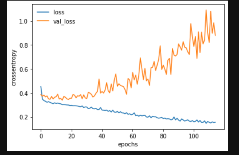
結果の確認（過学習モデル）

python.py

import matplotlib.pyplot as plt
%matplotlib inline
# グラフ表示
plt.plot(log.history['loss'], label='loss')
plt.plot(log.history['val_loss'], label='val_loss')
plt.legend(frameon=False) # 凡例の表示
plt.xlabel("epochs")
plt.ylabel("crossentropy")
plt.show()

python.py

# 正解率の確認
from sklearn.metrics import classification_report

Y_pred = model.predict_classes(X_test)
print(classification_report(y_test, Y_pred))

正解率:79%！！

早々に過学習しているかつ、正解率も低い状態。

過学習対策

過学習とは、「学習データの特徴を過度に学習したために、それ以外のデータ（検証データやテストデータ等）に対するモデルの性能が悪化した状態」。

つまり、与えたデータに適合しすぎて未知のデータについては全く対応できなくなってしまう状態のこと。

🌟過学習の主な原因：データに対してモデルが複雑すぎる。

🌟対策
・訓練データを増やす
・モデルのサイズを小さくする（単純なモデルにする）
・重みを正則化する
・ドロップアウトを追加する

過学習対策の実装

今回は、訓練データを増やすことはできないので、以下の3つをモデルに導入していきます。

・モデルのサイズを小さくする（単純なモデルにする）
・重みを正則化する
→「kernel_regularizer=keras.regularizers.l2(0.001)」
・ドロップアウトを追加する
→「model.add(Dropout(0.25))」（値は[0.25〜0.5]が一般的）

python.py

from tensorflow.keras.layers import Dropout

model = keras.Sequential()

#単純なモデルを構築

#入力層
model.add(Dense(32, kernel_regularizer=keras.regularizers.l2(0.001), activation = 'relu', input_shape=(12,)))

#中間層（隠れ層）
model.add(Dropout(0.25))
model.add(Dense(16, kernel_regularizer=keras.regularizers.l2(0.001), activation = 'relu'))
model.add(Dropout(0.25))
model.add(Dense(16, activation = 'relu'))
model.add(Dropout(0.5))
#出力層
model.add(Dense(1, activation = 'sigmoid'))

model.compile(optimizer = 'rmsprop', #オプティマイザー（誤差逆伝播法）
              loss = 'binary_crossentropy',#損失関数
              metrics = ['accuracy']) #訓練時に監視する指標

# 学習の実施
log = model.fit(X_train, y_train, 
                epochs=2000, #繰り返し計算する回数
                batch_size=512, #ミニバッチ勾配降下法で分割するデータかたまり
                verbose=2, #計算過程を表示
                callbacks=[keras.callbacks.EarlyStopping(monitor='val_loss', #監視する値
                                                         min_delta=0, #改善とみなされる最小の量
                                                         patience=100, #設定したエポック数改善がないと終了する
                                                         verbose=0)],
                validation_data=(X_valid, y_valid))

結果の確認（過学習対策モデル）

python.py

import matplotlib.pyplot as plt
%matplotlib inline
# グラフ表示
plt.plot(log.history['loss'], label='loss')
plt.plot(log.history['val_loss'], label='val_loss')
plt.legend(frameon=False) # 凡例の表示
plt.xlabel("epochs")
plt.ylabel("crossentropy")
plt.show()

python.py

# モデルの評価
from sklearn.metrics import classification_report

Y_pred = model.predict_classes(X_test)
print(classification_report(y_test, Y_pred))

 precision    recall  f1-score   support

           0       0.88      0.94      0.91      2446
           1       0.77      0.61      0.68       810

    accuracy                           0.86      3256
   macro avg       0.82      0.77      0.79      3256
weighted avg       0.85      0.86      0.85      3256

おわりに

過学習対策によって過学習の抑制と正解率の向上（79%→86%）しました！！