はじめに
Pythonを使った自然言語分析は、前処理用のパッケージのインストールに手間取ったり処理中にカーネルが止まってしまったりブルースクリーンが発生したりして私にとっては最も時間がかかる作業のひとつです。
Watson Discoveryにデータを投入してしまえば、辛い前処理から解放されて分析に集中することができます。さらに、Discovery Query Languageを使うことにより集計や結果の加工も行うことができるのです。
この記事では、以下のデータを使ってDiscovery Query Languageの使用例をご紹介します。
- 国土交通省 自動車の不具合・リコール情報 [データ1]
-
livedoor ニュースコーパス [データ2]
- トピックニュース
- Sports Watch
- IT ライフハック
※各カテゴリーを別コレクションへ投入
Discovery Query Languageとは
検索時に様々なパラメーターを組み合わせて1回の照会で複雑な検索や集計を可能にする非常に強力なクエリー言語で、API経由で実行できます。(Watson Discoveryのv1インスタンスではWeb UIから実行できましたが、v2ではメニューが無くなりました。)
検索の種類

自然言語照会は、文章による検索ができるためチャットボットとの親和性が高いです。ただし、入力全体が照会文として扱われるためAND ORのような演算子が有効にならないため注意が必要です。
照会言語検索はキーワードとAND OR 比較などの演算子の組み合わせによって検索されます。
いずれも結果は関連度の降順でソートされます。
検索オプション

ご参考: マニュアルリンク
Answer Findingは自然言語検索を行うときに使用できるベータ機能で、質問を解釈して単語や短文でのピンポイント回答を行います。ご参考Qiita記事: Answer Finding(Watson Discovery)のできること/できないこと
filterは条件抽出を行うオプションで、queryとは異なり結果のソートを行わないためqueryやaggregationの前処理として有用です。
検索APIの実行
ご参考:製品APIガイド
apikeyとurlの値はIBM Cloudのインスタンスのサービス資格情報を参照します。

project idはProjectを開き、Integrate and deploy > API Informationを押下して参照します。

cURLでの実行例
実行時に外部ファイルを読み込むことで、検索内容を変更しても同じコマンドを実行できるようにします。
実行コマンド [データ1]
curl -X POST \
-u "apikey:${apikey}” \
“${url}/v2/projects/${project_id}/query?version=2020-08-30“\
 -d @query_options.json -k -H "Content-Type: application/json"
検索処理設定ファイル
検索オプション名と値をJSON形式で記載します。
{
    “filter”: “走行不能”
    “aggregation”: ‘term(車名)’
}
Pythonでの実行例
Pythonで実行する場合、Watson API用パッケージのインストール→認証→検索の順に実行します。
Watson API用パッケージのインストール
pip install --upgrade "ibm-watson>=5.3.0"
認証
urlはIBM Cloudのサービス資格情報を参照し"instances"の前までを使用します。

from ibm_watson import DiscoveryV2
from ibm_cloud_sdk_core.authenticators import IAMAuthenticator
import json

authenticator = IAMAuthenticator(<apikey>)
discovery = DiscoveryV2(
    version='2020-08-30',
    authenticator=authenticator
)
discovery.set_service_url('<url>’)
検索 [データ1]
response = discovery.query(
  project_id='${project_id}',
  filter='走行不能',
  aggregation='term(車名)'
).get_result()
実行結果(抜粋)
"matching_result"は結果の件数です。
"aggregations"に集計結果が格納されます。今回は車名ごとの件数を集計しているため"field"に集計キーである「車名」、keyに車名フィールドの値、matching_resultsに件数が入っています。
"results"に検出された文書の情報が格納されます。"document_passages"は自然言語検索の結果にのみ値が挿入されます。
{
  "matching_results": 17129,
  "retrieval_details": {
    "document_retrieval_strategy": "untrained"
  },
  "aggregations": [
    {
      "type": "term",
      "field": "車名",
      "results": [
        {
          "key": "トヨタ",
          "matching_results": 2525
        },
  ],
  "results": [
    {
      "document_id": "d563095c2ef4d666230a7d2ea8b609e1_24001",
      "result_metadata": {
        "collection_id": "8b451f5a-7e6f-5547-0000-017d59d566fa"
      },
      "受付日": "2010-08-19T00:00:00Z",
      "document_passages": []
    },
  ]
}
Discovery Query Languageを活用した自然言語処理例
Pythonでの検索APIの実行と可視化の例をご紹介します。
以下の例ではPythonパッケージのインストールと認証の実行は割愛します。
例1: 特定のフィールドの値の出現頻度を集計し棒グラフとして表示 [データ1]
「修理」が含まれる文書数を性別をキーとして集計し、棒グラフとして表示します。
検索API実行
"filter"で"修理"が含まれる文書のみ抽出し、"aggregation"に"term(性別)"を指定することで性別ごとの件数を集計しています。
response = discovery.query(
  project_id=project_id,
  filter=‘修理',
  aggregation=‘term(性別)'
).get_result()
応答(抜粋)
"aggregation"の"results"以下の"key"が性別、"value"が文書数です。
"aggregations": [
    {
      "type": "term",
      "field": "性別",
      "results": [
        {
          "key": "男性",
          "matching_results": 356
        },
        {
          "key": "女性",
          "matching_results": 66
        },
描画
import matplotlib
import matplotlib.pyplot as plt

dept_name = [rec['key'] for rec in response['aggregations'][0]['results']]
dept_freq = [rec['matching_results'] for rec in response['aggregations'][0]['results']]
plt.rcParams["font.size"] = 40
plt.figure(figsize=(50,30))
plt.bar(dept_name,dept_freq)
plt.show()

例2: 特定のフィールドの値の出現頻度を集計しワードクラウドとして表示 [データ1]
「故障」に関する文書に含まれるキーワードを取得しワードクラウドを作成します。
検索API実行
「故障」に関する文書を"filter"で抽出、"term"でテキストに含まれるキーワードの出現頻度を集計、"count"で上位100件を取得します。
response = discovery.query(
  project_id=project_id,
  filter='故障',
  aggregation='term(
  enriched_申告内容の要約.keywords.text,
  count:100)'
).get_result()
応答(抜粋)
"results"以下の"key"がキーワード、"matching_results"が出現頻度です。
 "aggregations": [
    {
      "type": "term",
      "field": "enriched_申告内容の要約.keywords.text",
      "count": 100,
      "results": [
        {
          "key": "走行",
          "matching_results": 308
        },
        {
          "key": "エンジン",
          "matching_results": 174
        },
描画
import pandas as pd
from wordcloud import WordCloud
import matplotlib
import matplotlib.pyplot as plt

data = pd.DataFrame(response['aggregations'][0]['results'])
data = data.set_index(data['key'])['matching_results’]
wc = WordCloud(stopwords={‘故障’],
                                 font_path="/home/wsuser/.fonts/ipaexg.ttf",
                                 width=600,
                                 height=400)\
.generate_from_frequencies(data)
plt.figure(figsize=(100,100))
plt.imshow(wc)
plt.axis('off')
plt.show()

補足
キーワードの種類数を"unique_count"で集計し確認することでワードクラウドに表示する単語数(検索API実行時の"count"の値)を検討しやすくなります。
検索API実行
response = discovery.query(
  project_id='',
  filter='故障',
  aggregation=‘unique_count(
  enriched_申告内容の要約.keywords.text,
  )'
).get_result()
応答(抜粋)
"aggregations": [
    {
      "type": "unique_count",
      "field": "enriched_申告内容の要約.keywords.text",
      "value": 2003.0
    }
  ],
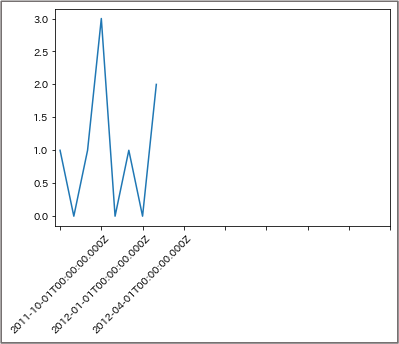
例3: 特定のキーワードに関する文書の数を時系列で集計しグラフとして表示 [データ2]
プロ野球に関する文書数を1ヵ月ごとに集計してグラフ化します。
検索API実行
"filter"で「プロ野球」が含まれる文書を抽出し、"timeslice"で時系列での集約を行っています。今回はタイムスタンプ型の"date"フィールドをもとに月ごとの文書数を取得しています。
response = discovery.query(
  project_id=project_id,
  filter='プロ野球’,
  aggregation='timeslice(date,1month)',
).get_result()
応答(抜粋)
"aggregations": [
    {
      "type": "timeslice",
      "field": "date",
      "interval": "1M",
      "results": [
        {
          "key": 1267401600000,
          "key_as_string": "2010-03-01T00:00:00.000Z",
          "matching_results": 2
        },
描画
import matplotlib
import matplotlib.pyplot as plt

plot_x = [result['key_as_string'] for result in response['aggregations'][0]['results']]
plot_y = [result['matching_results'] for result in response['aggregations'][0]['results’]]
plt.plot(plot_x,plot_y)
plt.xticks([0,3,6,9,12,15,18,21,24], rotation=45)

補足
検索API実行
先ほどの例ではプロジェクトの全文書を対象として条件抽出を行いましたが今度はコレクションをニュース・トピックのみに限定してスポーツ記事を除外します。
"collection_ids"にリスト形式でコレクションIDを指定することで検索対象を限定しています(プロジェクトに含まれないコレクションIDを指定するとエラーが発生するため注意が必要です)。
コレクションIDはwebコンソール上でコレクションを開き、"collections"と"activity"の間の値です。

response = discovery.query(
  project_id=project_id,
  collection_ids=[collection_id],
  filter='プロ野球’,
  aggregation='timeslice(date,1month)',
).get_result()
例4: 特定のフィールドの値のヒストグラムを表示 [データ1]
検索API実行
"filter"に複数の条件を指定しています。","はANDを意味します。"::"は左側のフィールドの値が右側と等しいことを示します。"|"はORです。つまり、「走行不能」かつ車名フィールドが「トヨタ」もしくは「ホンダ」の文書を抽出しています。
"histogram"はフィールドと間隔を指定して文書数を集計します。この例では総走行距離フィールドの値により10,000ごとに文書数を集計しています。
さらに、"histogram"の後ろに"term"を追加することによって車名ごとの集計結果を取得しています。
response = discovery.query(
  project_id=project_id,
  filter='走行不能,(車名::トヨタ|車名::ホンダ)',
  aggregation='histogram(\
                              総走行距離,\
                              interval:10000)\
                            .term(車名)',
).get_result()
応答(抜粋)
外側の"aggregations"の"key"に総走行距離の代表値(10,000ごとの値)が、"matching_results"に文書数が記載されています。さらに内側に"aggregations"があり"term"による車名ごとの集計結果が格納されています。
"aggregations": [
                    {
          "key": 10000,
          "matching_results": 295,
          "aggregations": [
            {
              "type": "term",
              "field": "車名",
              "results": [
                {
                  "key": "トヨタ",
                  "matching_results": 164
                },
                {
                  "key": "ホンダ",
                  "matching_results": 131
描画
複数の集計を実行した場合、結果の階層が深くなります。
また、該当文書数が0の場合は"matching_results"が0になるのではなく要素自体が作成されません。
複数系列の棒グラフを作成するときにはX軸とそれぞれの系列のY軸の値のリストの長さが同じである必要があります。今回は条件分岐により作成されなかった要素に0埋めしているためデータ加工部分の記述が長めになっています。
import matplotlib
import matplotlib.pyplot as plt

bin_list = []
value_list_toyota = []
value_list_honda = []
x_label_list = []
for aggregation in response['aggregations'][0]['results’]:
    bin_list.append(str(aggregation['key']))
    if aggregation['matching_results'] > 0:
        value_df = pd.DataFrame(aggregation['aggregations'][0]['results'])
        if len(value_df.loc[(value_df['key'] == 'トヨタ')]) > 0:
                value_list_toyota.append(int(value_df.loc[(value_df['key'] == 'トヨタ')]['matching_results']))
        else:
            value_list_toyota.append(0)

        if len(value_df.loc[(value_df['key'] == 'ホンダ')]) > 0:
                value_list_honda.append(int(value_df.loc[(value_df['key'] == 'ホンダ')]['matching_results']))
        else:
            value_list_honda.append(0)
    else:
        value_list_toyota.append(0)
        value_list_honda.append(0)

x_label_list = [round(int(dist)/10000) if int(dist)%50000 == 0  else '' for dist in bin_list]

plt.figure(figsize=(10,8))
plt.bar(bin_list,value_list_toyota,width=-0.5,align='edge')
plt.bar(bin_list,value_list_honda,width=0.5,align='edge’)
plt.xticks(bin_list,x_label_list)

補足
検索API実行
数値項目は比較演算子による条件の設定も可能です。今回は総走行距離が200,000以上のみ抽出します。
response = discovery.query(
  project_id=project_id,
  filter='走行不能,総走行距離>=200000,(車名::トヨタ|車名::ホンダ)’,
  aggregation='histogram(\
                              総走行距離,\
                              interval:10000)\
                            .term(車名)',
).get_result()

例5: 特定のフィールドの値別に別のフィールドの値の平均値と上位1件の元文書を取得 [データ1]
検索API実行
"filter"により走行不能が含まれる文書を抽出します。"term"と"average"を組み合わせて不具合装置別の平均総走行距離を出すとともに不具合装置ごとに関連度が1位の文書を取得します。
response = discovery.query(
  project_id=project_id,
  filter='走行不能',
  aggregation='term(不具合装置)\
                            .average(総走行距離)\
                            .top_hits(1)'
).get_result()
応答(抜粋)
"results"内の内側の"aggregations"が不具合装置別の上位1件の元文書("hits")と平均総走行距離("value": 72729.44614404079)です。
"aggregations": [
    {
      "type": "term",
      "field": "不具合装置",
      "results": [
        {
          "key": "エンジン",
          "matching_results": 5644,
          "aggregations": [
            {
              "type": "top_hits",
              "size": 1,
              "hits": {
                "matching_results": 5644,
                "hits": [
                  {
                    "申告内容の要約": [
                      "実走行4000km余りでエンジンマウントが劣化した。"
                    ],
                    "            {
              "type": "average",
              "field": "総走行距離",
              "value": 72729.44614404079
            }
          ]
        },
例6: 検索結果のソート [データ2]
デフォルトでは"query"の結果は関連度順にソートされますが、任意のフィールドの値でソートすることもできます。
検索API実行
"sort='-受付日'"で受付日フィールドの値による降順(-)ソートを指定しています。
# ソートなし
response = discovery.query(
  project_id=project_id,
  query='エンジン,故障',
  count=30,
).get_result()

# ソートあり
response = discovery.query(
  project_id=project_id,
  query='エンジン,故障',
  count=30,
  sort=‘-受付日’
).get_result()
応答(抜粋)
# ソートなしの場合の"results"の先頭
"受付日": "2011-02-06T15:00:00Z",

"申告内容の要約": [
        "アイドルスピードコントロールバルブが故障し、
        その故障による異常電流でエンジンコンピューターまで故障したため、
        走行中にエンジンが停止し、再始動不能になった。"

# ソートありの場合の"results"の先頭
"受付日": "2015-12-07T15:00:00Z",

"申告内容の要約": [
        "SMT(シーケンシャルトランスミッション)の故障により、
    警告灯が点いて走行中にエンジンが停止した。"
例7: 上位N件を除外した結果を取得 [データ2]
あえて関連度が高い結果を外して気付きを得たいときに使える関数です。
検索API実行
"offset"に除外したい文書数を指定します。
# 除外オプションなし
response = discovery.query(
  project_id=project_id,
  query=‘W杯,サッカー',
  return_=['document_passages.passage_text'],
).get_result()

# 除外オプションあり
response = discovery.query(
  project_id=project_id,
  query=‘W杯,サッカー',
  return_=['document_passages.passage_text’],
  offset=20
).get_result()
例8: 単語または単文での回答の取得(Answer Finding) [データ2]
Answer Findingについては以下もご参照ください。
Anwer Finding(Watson Discovery)のできること/できないこと
検索API実行
"natural_language_query"で検索を行い、"passages"以下の"enabled"と"find_answers"を'true'にします。"fields"は答えの抽出元となるフィールドを、"characters"は答えの抽出元となる文書の一部分の長さを指定するパラメーターです。
response = discovery.query(
  project_id = project_id,
  natural_language_query=\
  '2011年に生まれた男の子の名前の1位は’,
  passages={
  "enabled": 'true’,
  "find_answers":'true’,
  "fields":['body’],
  “characters”:100
  }
).get_result()
応答(抜粋)
"answer_text"が回答です。
"document_passages": [
        {
          "passage_text": “……",
          "start_offset": 0,
          "end_offset": 200,
          "field": "body",
          "answers": [
            {
              "answer_text": "大翔",
              "start_offset": 95,
              "end_offset": 97,
              "confidence": 0.98137116
おわりに
上記の使用例からわかるように、Watson Discoveryを活用することで自然言語の前処理を作業端末上で行う必要がなくなります。さらに、検索APIを使うことで集計処理からも解放され描画や結果の理解に時間を使うことができるようになりました。体感的には自然言語の分析にかかる手間や時間が2割くらいになりました(個人の感想です)。
お断り
このサイトの掲載内容は私自身の見解であり、必ずしも所属会社の立場、戦略、意見を代表するものではありません。 記事は執筆時点の情報を元に書いているため、必ずしも最新情報であるとはかぎりません。 記事の内容の正確性には責任を負いません。自己責任で実行してください。