はじめに
時系列データの予測の勉強として、東京電力(TEPCO)の電力需給実績データを題材に、ARMA・ARMAX・LightGBMの3モデルを実装・比較し、それぞれの特性を考察する。
データ
データソース
東京電力パワーグリッド 需給実績データを使用する。2016年度〜2026年3月の日次平均需要(MW)を対象とする。
| 項目 | 内容 |
|---|---|
| 期間 | 2016/04/01 〜 2026/03/31 |
| 単位 | 日次平均(MW) |
| 学習期間 | 2016/04/01 〜 2025/03/31(3,287日) |
| 検証期間 | 2025/04/01 〜 2026/03/31(365日) |
前処理上の注意点
TEPCOのデータは2024年2月を境にフォーマットが変わっており、旧形式(万kW)と新形式(MW)で単位が異なる。1万kW = 10,000kW = 10MWなので、旧形式に10を乗じてMWに統一する。
モデルと手法
1. ベースライン:月×曜日の過去平均
学習期間中の同じ月・曜日の組み合わせの平均値を予測値とする。例えば「1月の月曜日」であれば、学習期間中の1月の月曜日の需要の平均値を使う。これにより曜日・月の季節性を考慮した上で、時系列モデルとの公平な比較を行う。
2. ARMA(p, q)
ADF検定によりこのデータの定常性を確認した(ADF統計量 = −6.81、p値 < 0.001)ため、まずはARMA(自己回帰移動平均)モデルを用いる。過去の観測値と過去の誤差の線形結合で現在値を予測する。
$$
y_t = c + \sum_{i=1}^{p} \phi_i y_{t-i} + \sum_{j=1}^{q} \theta_j \varepsilon_{t-j} + \varepsilon_t
$$
- $\phi_i$:AR係数(過去の需要の影響)
- $\theta_j$:MA係数(過去の撹乱項の影響)
- $\varepsilon_t$:ホワイトノイズ
ARMAは定常時系列を前提とする。
AICを最小化するようにグリッドサーチ($p \in {1,...,7}$、$q \in {0,...,3}$)で次数を選択した結果、ARMA(7, 3) が選ばれた。
ウォークフォワード検証
検証期間では毎日1ステップ先を予測し、実績値を逐次追加する walk-forward 評価を行う。
3. ARMAX(p, q)
ARMAX(外生変数付きARMA)は、ARMAに外生変数ベクトル $\mathbf{x}_t$ を加えたモデルである。
$$
y_t = c + \sum_{i=1}^{p} \phi_i y_{t-i} + \sum_{j=1}^{q} \theta_j \varepsilon_{t-j} + \boldsymbol{\beta}^\top \mathbf{x}_t + \varepsilon_t
$$
以下を外生変数として使用した。
| 変数 | 内容 | 列数 |
|---|---|---|
| 曜日ダミー | 月曜を基準に火〜日の6列 | 6 |
| 月ダミー | 1月を基準に2〜12月の11列 | 11 |
グリッドサーチの結果、ARMAX(3, 0) が選ばれた。
推定された係数
y_t = +36675.1
  +0.8667 * y_{t-1}
  -0.1099 * y_{t-2}
  +0.0420 * y_{t-3}
  +856.7  * dow_1(火曜)
  +749.2  * dow_2(水曜)
  +689.7  * dow_3(木曜)
  +564.3  * dow_4(金曜)
  -2362.9 * dow_5(土曜)
  -3830.0 * dow_6(日曜)
  -8865.3 * month_5(5月)
  -7713.8 * month_4(4月)
  +452.6  * month_8(8月)
  ...
  + ε_t
曜日効果(基準:月曜):火〜金は月曜より800MW前後高く、土曜は約2,363MW、日曜は約3,830MW低い。週末の需要減少は、休日となる企業が多いことから納得感がある。
月効果(基準:1月):春・秋(4〜5月、10〜11月)に需要が低下し、1月・8月付近でピークとなるU字型の季節性が確認できる。
4. LightGBM
勾配ブースティング決定木(GBDT)モデルとして LightGBM を使用する。以下の特徴量を作成した。
| 特徴量 | 内容 |
|---|---|
lag_1 〜 lag_7
|
1〜7日前の需要 |
ma_1_1 〜 ma_1_7
|
直近1〜7日間の移動平均需要 |
month |
月(1〜12) |
dayofweek |
曜日(0〜6) |
結果
精度比較
| モデル | MAE (MW) | RMSE (MW) | MAPE (%) |
|---|---|---|---|
| Baseline(月×曜日平均) | 2,553.7 | 3,225.6 | 8.01 |
| ARMA(7, 3) | 1,488.1 | 1,916.3 | 4.62 |
| ARMAX(3, 0) | 1,283.0 | 1,755.7 | 4.00 |
| LightGBM | 1,268.8 | 1,700.8 | 3.94 |
予測と残差(一部抜粋)
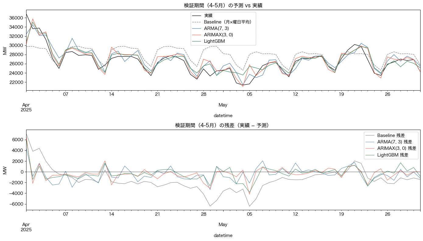
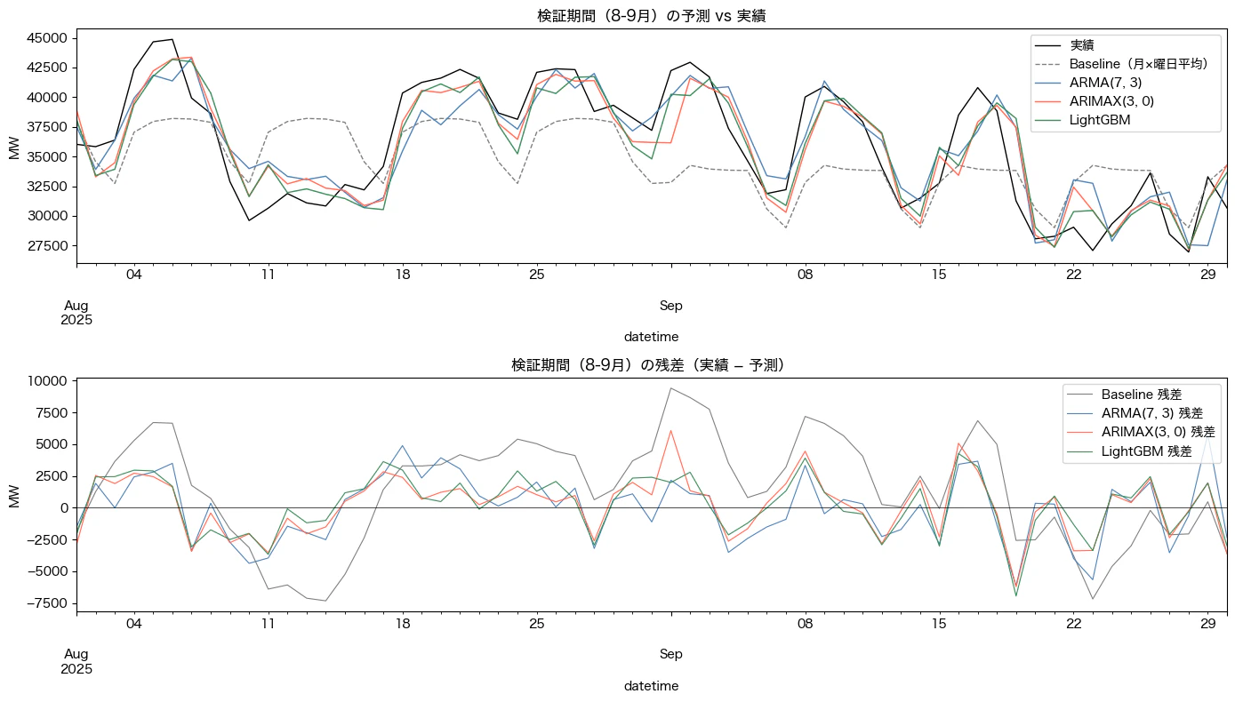
考察
ARMAはベースラインを大幅に上回る。過去の需要値の自己相関を利用するだけで、季節性を考慮したナイーブ予測を大きく上回ることが確認できた。
ARMAXで曜日・月を外生変数として加えると精度がさらに改善する。MAEで約205MW(約14%)の改善となった。重要なのは、この改善が「係数として直接解釈できる」点である。「日曜は月曜比3,830MW減」といった形で、予測根拠を説明しやすい。
LightGBMとARMAXの精度差はほぼない。MAEの差は約14MW(1%未満)に過ぎない。ARMAXで十分データ生成仮定が再現される場合は、LightGBMにすることによる改善幅は小さい。
ただし、この状況はLightGBMにとって条件が良くない。LightGBMは特徴量の追加やハイパーパラメータチューニングによってさらに精度を伸ばせる余地が大きい。気温データの追加は特に効果が期待でき、夏・冬の需要ピークを直接説明できる特徴量になる。
実務上は以下のように使い分けが考えられる。
| 優先事項 | 推奨モデル |
|---|---|
| 手頃なベースライン | (S)AR(I)MAX |
| 予測精度の最大化 | LightGBM(特徴量増加・チューニング込み) |
| 手軽なベースライン | ARMA |
今後
今回は、予測精度のみが論点となったが、実務ではまず課題が先にあり、その解決の手段として統計・機械学習が使われるので、その課題の性質を踏まえたモデル構築が必要となる。
参考
サンプルコード
データ取得
import time
from pathlib import Path

import pandas as pd
import requests

RAW_DIR = Path("data/raw")
(RAW_DIR / "tepco").mkdir(parents=True, exist_ok=True)
(RAW_DIR / "holiday").mkdir(parents=True, exist_ok=True)

# 旧形式: 2016〜2023年度(万kW、年度別CSV)
for year in range(2016, 2024):
    path = RAW_DIR / "tepco" / f"area-{year}.csv"
    if path.exists():
        continue
    resp = requests.get(f"https://www.tepco.co.jp/forecast/html/images/area-{year}.csv", timeout=15)
    if resp.status_code == 200:
        path.write_bytes(resp.content)
    time.sleep(0.5)

# 新形式: 2024/02〜(MW、月別CSV)
for month in pd.date_range(start="2024-02-01", end=pd.Timestamp.today(), freq="MS"):
    yyyymm = month.strftime("%Y%m")
    path = RAW_DIR / "tepco" / f"eria_jukyu_{yyyymm}_03.csv"
    if path.exists():
        continue
    resp = requests.get(
        f"https://www.tepco.co.jp/forecast/html/images/eria_jukyu_{yyyymm}_03.csv", timeout=15
    )
    if resp.status_code == 200:
        path.write_bytes(resp.content)
    time.sleep(0.5)

# 内閣府 祝日CSV
holiday_path = RAW_DIR / "holiday" / "syukujitsu.csv"
if not holiday_path.exists():
    resp = requests.get("https://www8.cao.go.jp/chosei/shukujitsu/syukujitsu.csv", timeout=10)
    resp.raise_for_status()
    holiday_path.write_bytes(resp.content)
データクレンジング
from pathlib import Path

import pandas as pd

RAW_DIR = Path("data/raw")
INTERIM_DIR = Path("data/interim")
PROCESSED_DIR = Path("data/processed")
INTERIM_DIR.mkdir(parents=True, exist_ok=True)
PROCESSED_DIR.mkdir(parents=True, exist_ok=True)

# 旧形式の読み込み(shift-jis、万kW → MW に10倍変換)
def load_area_csv(filepath: Path) -> pd.Series:
    df = pd.read_csv(filepath, encoding="shift-jis", skiprows=2, header=0, thousands=",")
    df = df.iloc[:, :3]
    df.columns = ["DATE", "TIME", "demand_mw"]
    df["demand_mw"] = pd.to_numeric(df["demand_mw"], errors="coerce") * 10  # 万kW → MW
    df["datetime"] = pd.to_datetime(df["DATE"] + " " + df["TIME"], errors="coerce")
    return df.dropna(subset=["datetime"]).set_index("datetime")["demand_mw"]

old_series = pd.concat([
    load_area_csv(p) for p in sorted((RAW_DIR / "tepco").glob("area-*.csv"))
])

# 新形式の読み込み(utf-8、MW)
def load_eria_csv(filepath: Path) -> pd.Series:
    df = pd.read_csv(filepath, encoding="utf-8", skiprows=1)
    df.columns = df.columns.str.strip()
    df["datetime"] = pd.to_datetime(df.iloc[:, 0] + " " + df.iloc[:, 1], errors="coerce")
    demand_col = [c for c in df.columns if "エリア需要" in c][0]
    return df.dropna(subset=["datetime"]).set_index("datetime")[demand_col].rename("demand_mw")

new_series = pd.concat([
    load_eria_csv(p) for p in sorted((RAW_DIR / "tepco").glob("eria_jukyu_*.csv"))
])

# 重複除去(新形式優先)・日次平均に集計
combined = pd.concat([old_series, new_series])
combined = combined[~combined.index.duplicated(keep="last")].sort_index()
tepco_daily = combined.resample("D").mean().rename("demand_mw").to_frame()
tepco_daily.to_csv(INTERIM_DIR / "tepco_daily.csv")

# 祝日データ
holiday_raw = pd.read_csv(RAW_DIR / "holiday" / "syukujitsu.csv", encoding="shift-jis", header=0)
holiday_raw.columns = ["date", "name"]
holiday_raw["date"] = pd.to_datetime(holiday_raw["date"], format="%Y/%m/%d", errors="coerce")
holiday = holiday_raw.dropna(subset=["date"]).set_index("date").sort_index()
holiday.to_csv(INTERIM_DIR / "holiday.csv")

# 特徴量結合
tepco_daily = pd.read_csv(INTERIM_DIR / "tepco_daily.csv", index_col=0, parse_dates=True)
holiday = pd.read_csv(INTERIM_DIR / "holiday.csv", index_col=0, parse_dates=True)
holiday_set = set(holiday.index.date)

tepco_daily["is_holiday"]    = [int(d in holiday_set) for d in tepco_daily.index.date]
tepco_daily["dayofweek"]     = tepco_daily.index.dayofweek
tepco_daily["is_weekend"]    = (tepco_daily["dayofweek"] >= 5).astype(int)
tepco_daily["month"]         = tepco_daily.index.month
tepco_daily["is_nonworking"] = ((tepco_daily["is_weekend"] == 1) | (tepco_daily["is_holiday"] == 1)).astype(int)
tepco_daily.to_csv(PROCESSED_DIR / "daily_features.csv")
分析
from pathlib import Path

import lightgbm as lgb
import matplotlib.pyplot as plt
import numpy as np
import pandas as pd
from statsmodels.tsa.arima.model import ARIMA

df = pd.read_csv(Path("data/processed/daily_features.csv"), index_col=0, parse_dates=True)

TRAIN_START, TRAIN_END = "2016-04-01", "2025-03-31"
VAL_START,   VAL_END   = "2025-04-01", "2026-03-31"

train = df.loc[TRAIN_START:TRAIN_END, "demand_mw"].dropna()
val   = df.loc[VAL_START:VAL_END,     "demand_mw"].dropna()

exog = pd.concat([
    pd.get_dummies(df["dayofweek"], prefix="dow",   drop_first=True),
    pd.get_dummies(df["month"],     prefix="month", drop_first=True),
], axis=1).astype(float)
exog_train = exog.loc[TRAIN_START:TRAIN_END].loc[train.index]
exog_val   = exog.loc[VAL_START:VAL_END].loc[val.index]

# ベースライン: 月×曜日の平均
train_df = train.to_frame("demand_mw")
train_df["month"], train_df["dayofweek"] = train_df.index.month, train_df.index.dayofweek
monthly_dow_mean = train_df.groupby(["month", "dayofweek"])["demand_mw"].mean()
baseline_pred = pd.Series(
    [monthly_dow_mean.loc[(d.month, d.dayofweek)] for d in val.index],
    index=val.index,
)

# ARMA: AICによる次数選択 + ウォークフォワード予測
best_aic, best_order = np.inf, (1, 0)
for p in range(1, 8):
    for q in range(0, 4):
        try:
            aic = ARIMA(train, order=(p, 0, q)).fit().aic
            if aic < best_aic:
                best_aic, best_order = aic, (p, q)
        except Exception:
            pass
P_arma, Q_arma = best_order

fitted = ARIMA(train, order=(P_arma, 0, Q_arma)).fit()
arma_preds = []
for date, actual in val.items():
    arma_preds.append(fitted.forecast(steps=1).iloc[0])
    fitted = fitted.append([actual])
arma_pred = pd.Series(arma_preds, index=val.index)

# ARMAX: AICによる次数選択 + ウォークフォワード予測
best_aic, best_order = np.inf, (1, 0)
for p in range(1, 8):
    for q in range(0, 4):
        try:
            aic = ARIMA(train, exog=exog_train, order=(p, 0, q)).fit().aic
            if aic < best_aic:
                best_aic, best_order = aic, (p, q)
        except Exception:
            pass
P_arimax, Q_arimax = best_order

fitted = ARIMA(train, exog=exog_train, order=(P_arimax, 0, Q_arimax)).fit()
arimax_preds = []
for i, (date, actual) in enumerate(val.items()):
    arimax_preds.append(fitted.forecast(steps=1, exog=exog_val.iloc[[i]]).iloc[0])
    fitted = fitted.append([actual], exog=exog_val.iloc[[i]])
arimax_pred = pd.Series(arimax_preds, index=val.index)

# LightGBM
def build_features(series: pd.Series) -> pd.DataFrame:
    df_feat = pd.DataFrame({"demand_mw": series})
    for i in range(1, 8):
        df_feat[f"lag_{i}"]  = series.shift(i)
        df_feat[f"ma_1_{i}"] = series.shift(1).rolling(i).mean()
    df_feat["month"]     = series.index.month
    df_feat["dayofweek"] = series.index.dayofweek
    return df_feat

df_feat  = build_features(df.loc["2016-04-01":VAL_END, "demand_mw"].dropna()).dropna()
FEAT_COLS = [c for c in df_feat.columns if c != "demand_mw"]
X_train, y_train = df_feat.loc[TRAIN_START:TRAIN_END, FEAT_COLS], df_feat.loc[TRAIN_START:TRAIN_END, "demand_mw"]
X_val,   y_val   = df_feat.loc[VAL_START:VAL_END,     FEAT_COLS], df_feat.loc[VAL_START:VAL_END,     "demand_mw"]

lgb_model = lgb.LGBMRegressor(n_estimators=500, learning_rate=0.05, num_leaves=31, random_state=42, verbose=-1)
lgb_model.fit(X_train, y_train, eval_set=[(X_val, y_val)], callbacks=[lgb.early_stopping(50, verbose=False)])
lgb_pred = pd.Series(lgb_model.predict(X_val), index=X_val.index)

# 精度評価
def evaluate(actual, pred, name):
    mae  = np.mean(np.abs(actual - pred))
    rmse = np.sqrt(np.mean((actual - pred) ** 2))
    mape = np.mean(np.abs((actual - pred) / actual)) * 100
    return {"name": name, "MAE": mae, "RMSE": rmse, "MAPE": mape}

val_aligned = val.loc[val.index.intersection(lgb_pred.index)]
results = [
    evaluate(val,         baseline_pred,              "Baseline(月×曜日平均)"),
    evaluate(val,         arma_pred,                  f"ARMA({P_arma}, {Q_arma})"),
    evaluate(val,         arimax_pred,                f"ARMAX({P_arimax}, {Q_arimax})"),
    evaluate(val_aligned, lgb_pred.loc[val_aligned.index], "LightGBM"),
]
print(pd.DataFrame(results).set_index("name").to_string())