はじめに
この記事は Aidemy Premium plan AIアプリ開発コースの最終成果物として AIを用いた画像認
識アプリを開発する過程を記録したものです。
元々バイク屋におり現在もバイクを使用する仕事についておりAIで同じような形ばかりの
バイクをどこまで判別できるのかが気になりこの課題にしました。
目次
1. 実行環境
2. 画像の収集
3. 画像のリサイズ
4. CNNモデル作成および学習
5. HTMLとFlaskコードの作成
6. アプリの動作確認
7. 改善点
8. 結果
1.実行環境
・Visual Studio Code
・Google Colaboratory
2.画像の収集
バイクはパッと見たところ外観に変化があまりなく車両に大量にステッカーを貼って
いるものも多く判別しにくいかもと思い今回は手動で集めました。
集めた車両は
・KAWASAKI:zx10R
・SUZUKI:刀
・YAMAHA:VMAX
・HONDA:CB1100R
・Harley-Davidson:XL1200
各バイク50枚ずつ集めました。
GoogleDrive上に画像を保管する場合はドライブをマウントしなければなりません。
以下のコードを実行することで、マウントできます。
from google.colab import drive
drive.mount('/content/drive')
3.画像のリサイズと水増し
import os
import cv2
import numpy as np
import matplotlib.pyplot as plt
from tensorflow.keras.utils import to_categorical
from tensorflow.keras.layers import Dense, Dropout, Flatten, Input
from tensorflow.keras.applications.vgg16 import VGG16
from tensorflow.keras.models import Model, Sequential
from tensorflow.keras import optimizers
from tensorflow.keras.preprocessing.image import ImageDataGenerator
from tensorflow.keras.preprocessing.image import img_to_array

# リサイズ関数
def resize_image(input_path, output_path, new_width, new_height):
    image = cv2.imread(input_path)
    resized_image = cv2.resize(image, (new_width, new_height))
    cv2.imwrite(output_path, resized_image)

# リサイズするフォルダと出力フォルダのリストを指定
folders_to_resize = ['/content/drive/MyDrive/kadai3/ZX10R/', '/content/drive/MyDrive/kadai3/CB1100R/', '/content/drive/MyDrive/kadai3/VMAX/', '/content/drive/MyDrive/kadai3/KATANA/', '/content/drive/MyDrive/kadai3/XL1200/']
output_folders = ['/content/drive/MyDrive/kadai3/OUT_ZX10R/', '/content/drive/MyDrive/kadai3/OUT_CB1100R/', '/content/drive/MyDrive/kadai3/OUT_VMAX/', '/content/drive/MyDrive/kadai3/OUT_KATANA/', '/content/drive/MyDrive/kadai3/OUT_XL1200/']

# 新しいサイズを指定
new_width = 150
new_height = 150

# 画像のリサイズ
for i in range(len(folders_to_resize)):
    input_folder = folders_to_resize[i]
    output_folder = output_folders[i]
    if not os.path.exists(output_folder):
        os.makedirs(output_folder)

    for filename in os.listdir(input_folder):
        if filename.endswith(('.jpg', '.jpeg', '.png', '.bmp')):
            input_path = os.path.join(input_folder, filename)
            output_path = os.path.join(output_folder, filename)
            resize_image(input_path, output_path, new_width, new_height)

# データ拡張用のImageDataGenerator
datagen = ImageDataGenerator(
    rotation_range=90, # 90°まで回転
    width_shift_range=0.1, # 水平方向にランダムでシフト
    height_shift_range=0.1, # 垂直方向にランダムでシフト
    channel_shift_range=50.0, # 色調をランダム変更
    shear_range=0.39, # 斜め方向(pi/8まで)に引っ張る
    horizontal_flip=True, # 垂直方向にランダムで反転
    vertical_flip=True # 水平方向にランダムで反転
)

# 画像フォルダのリスト
image_folders =  ['/content/drive/MyDrive/kadai3/OUT_ZX10R/', '/content/drive/MyDrive/kadai3/OUT_CB1100R/', '/content/drive/MyDrive/kadai3/OUT_VMAX/', '/content/drive/MyDrive/kadai3/OUT_KATANA/', '/content/drive/MyDrive/kadai3/OUT_XL1200/']

for folder in image_folders:
    for filename in os.listdir(folder):
        if filename.endswith(('.jpg', '.jpeg', '.png', '.bmp')):
            img_path = os.path.join(folder, filename)
            img = cv2.imread(img_path)
            x = img_to_array(img)
            x = x.reshape((1,) + x.shape)

            i = 0
            for batch in datagen.flow(x, batch_size=1):
                plt.figure(i)
                imgplot = plt.imshow(batch[0].astype(int))  # OpenCVイメージを正しく表示するためにastype(int)を追加
                i += 1
                if i % 4 == 0:
                    break

plt.show()
収集した画像にはサイズの違いが大きくそのまま学習させようとするとメモリ不足になったり学習させるのに時間がかかったりといいことがないので、リサイズします。
水増しをする理由としてトレーニングデータの多様性が増し、過学習防止の手助けとなります。
そのほかにデータ変換(回転、シフト、反転、明るさの変更)により、モデル画像がたくさんあるように認識させます。
4.CNNモデル作成および学習
import os
import cv2
import numpy as np
import matplotlib.pyplot as plt
from tensorflow.keras.applications.vgg16 import VGG16
from tensorflow.keras.layers import GlobalAveragePooling2D, Dense, Dropout
from tensorflow.keras.models import Model
from tensorflow.keras.optimizers import Adam
from tensorflow.keras.utils import to_categorical
from sklearn.model_selection import train_test_split
from sklearn.metrics import classification_report, confusion_matrix

# 画像が格納されているディレクトリ
data_dir = '/content/drive/MyDrive/kadai3/'

# クラスラベルとディレクトリの対応
class_labels = {
    'ZX10R': 0,
    'KATANA': 1,
    'CB1100R': 2,
    'VMAX': 3,
    'XL1200': 4
}

# 画像データとクラスラベルを格納するリスト
X = []
y = []

# ディレクトリごとに画像を読み込んでリストに追加
for class_label, class_id in class_labels.items():
    class_dir = os.path.join(data_dir, class_label)
    for image_file in os.listdir(class_dir):
        if image_file.endswith(".jpg"):
            image_path = os.path.join(class_dir, image_file)
            image = cv2.imread(image_path)
            image = cv2.resize(image, (224, 224))
            X.append(image)
            y.append(class_id)

# リストをNumPy配列に変換
X = np.array(X)
y = np.array(y)

# データをシャッフル
shuffle_indices = np.arange(X.shape[0])
np.random.shuffle(shuffle_indices)
X = X[shuffle_indices]
y = y[shuffle_indices]

# データの正規化
X = X.astype('float32') / 255.0

# クラスラベルをワンホットエンコーディング
y = to_categorical(y, num_classes=5)

# データを訓練データとテストデータに分割
X_train, X_test, y_train, y_test = train_test_split(X, y, test_size=0.2, random_state=42)

# データ拡張用のImageDataGenerator
from tensorflow.keras.preprocessing.image import ImageDataGenerator

datagen = ImageDataGenerator(
    rotation_range=40,
    width_shift_range=0.2,
    height_shift_range=0.2,
    shear_range=0.2,
    zoom_range=0.2,
    horizontal_flip=True,
    fill_mode='nearest')

# VGG16モデルの読み込み
base_model = VGG16(weights='imagenet', include_top=False, input_shape=(224, 224, 3))

# ベースモデルから一部の畳み込み層を削除(例: 後ろから3つの畳み込み層を削除)
for _ in range(3):
    base_model.layers.pop()

# ベースモデルの一部の層をフリーズ
for layer in base_model.layers:
    layer.trainable = False

x = base_model.output
x = GlobalAveragePooling2D()(x)
x = Dense(128, activation='relu')(x)  # Dense層のユニット数を減らす
x = Dropout(0.5)(x)  # ドロップアウトを追加

# 最終的な出力層を追加
predictions = Dense(5, activation='softmax')(x)

model = Model(inputs=base_model.input, outputs=predictions)

# モデルの訓練
model.compile(optimizer=Adam(learning_rate=0.01), loss='categorical_crossentropy', metrics=['accuracy'])

# 早期停止のコールバックを追加
from tensorflow.keras.callbacks import EarlyStopping

early_stopping = EarlyStopping(monitor='val_loss', patience=5, restore_best_weights=True)

history = model.fit(X_train, y_train, batch_size=50, epochs=15, validation_data=(X_test, y_test), callbacks=[early_stopping])


# モデル評価
test_scores = model.evaluate(X_test, y_test, verbose=0)
print("Test loss:", test_scores[0])
print("Test accuracy:", test_scores[1])

# 混同行列と評価数値を表示
y_pred = model.predict(X_test)
y_pred_classes = np.argmax(y_pred, axis=1)
y_true = np.argmax(y_test, axis=1)

confusion_mtx = confusion_matrix(y_true, y_pred_classes)
print(confusion_mtx)
print(classification_report(y_true, y_pred_classes))

# 評価グラフの作成
plt.figure(figsize=(12, 4))
plt.subplot(1, 2, 1)
plt.plot(history.history['accuracy'], label='Train')
plt.plot(history.history['val_accuracy'], label='Validation')
plt.title('Model accuracy')
plt.xlabel('Epoch')
plt.ylabel('Accuracy')
plt.legend()

plt.subplot(1, 2, 2)
plt.plot(history.history['loss'], label='Train')
plt.plot(history.history['val_loss'], label='Validation')
plt.title('Model loss')
plt.xlabel('Epoch')
plt.ylabel('Loss')
plt.legend()

plt.show()

# モデルの保存
model.save("modell.h5")
# ディレクトリごとに画像を読み込んでリストに追加
for class_label, class_id in class_labels.items():
    class_dir = os.path.join(data_dir, class_label)
    for image_file in os.listdir(class_dir):
        if image_file.endswith(".jpg"):
            image_path = os.path.join(class_dir, image_file)
            image = cv2.imread(image_path)
            image = cv2.resize(image, (224, 224))
            X.append(image)
            y.append(class_id)

# リストをNumPy配列に変換
X = np.array(X)
y = np.array(y)

# データをシャッフル
shuffle_indices = np.arange(X.shape[0])
np.random.shuffle(shuffle_indices)
X = X[shuffle_indices]
y = y[shuffle_indices]

# データの正規化
X = X.astype('float32') / 255.0

# クラスラベルをワンホットエンコーディング
y = to_categorical(y, num_classes=5)

# データを訓練データとテストデータに分割
X_train, X_test, y_train, y_test = train_test_split(X, y, test_size=0.2, random_state=42)

# データ拡張用のImageDataGenerator
from tensorflow.keras.preprocessing.image import ImageDataGenerator

datagen = ImageDataGenerator(
    rotation_range=40,
    width_shift_range=0.2,
    height_shift_range=0.2,
    shear_range=0.2,
    zoom_range=0.2,
    horizontal_flip=True,
    fill_mode='nearest')
画像が格納されているディレクトリとそれに対応するクラスラベル(クラス名と対応する数値)を設定します。
画像データとクラスラベルを格納するためのリスト X と y を用意します。
各クラスのディレクトリ内にある画像を読み込み、指定されたサイズ(ここでは224x224ピクセル)にリサイズします。
画像データをリスト X に追加し、対応するクラスラベルをリスト y に追加します。
画像データをNumPy配列に変換し、0から1の範囲に正規化します。
このデータ拡張は、モデルの入力データとして使用され、訓練中にミニバッチごとに適用される。
# VGG16モデルの読み込み
base_model = VGG16(weights='imagenet', include_top=False, input_shape=(224, 224, 3))

# ベースモデルから一部の畳み込み層を削除(例: 後ろから3つの畳み込み層を削除)
for _ in range(3):
    base_model.layers.pop()

# ベースモデルの一部の層をフリーズ
for layer in base_model.layers:
    layer.trainable = False

x = base_model.output
x = GlobalAveragePooling2D()(x)
x = Dense(128, activation='relu')(x)
x = Dropout(0.5)(x)  # ドロップアウトを追加

# 最終的な出力層を追加
predictions = Dense(5, activation='softmax')(x)

model = Model(inputs=base_model.input, outputs=predictions)

# モデルの訓練
model.compile(optimizer=Adam(learning_rate=0.01), loss='categorical_crossentropy', metrics=['accuracy'])

# 早期停止のコールバックを追加
from tensorflow.keras.callbacks import EarlyStopping

early_stopping = EarlyStopping(monitor='val_loss', patience=5, restore_best_weights=True)

history = model.fit(X_train, y_train, batch_size=50, epochs=15, validation_data=(X_test, y_test), callbacks=[early_stopping])


# モデル評価
test_scores = model.evaluate(X_test, y_test, verbose=0)
print("Test loss:", test_scores[0])
print("Test accuracy:", test_scores[1])

# 混同行列と評価数値を表示
y_pred = model.predict(X_test)
y_pred_classes = np.argmax(y_pred, axis=1)
y_true = np.argmax(y_test, axis=1)

confusion_mtx = confusion_matrix(y_true, y_pred_classes)
print(confusion_mtx)
print(classification_report(y_true, y_pred_classes))
VGG16モデルを読み込みます。このモデルは、事前学習済みの特徴抽出器として使用されます。
ベースモデルから一部の畳み込み層を削除し、一部の層を凍結します。その後、新しい全結合層(Dense層)と最終的な出力層を追加します。最終的な出力層は5つのクラスに対応しており、softmax活性化関数が使用されます。
モデルの訓練を行います。訓練データを使用してモデルを学習し、検証データを使用してモデルの性能を監視します。
Adamオプティマイザとカテゴリカル交差エントロピー損失関数を使用して、モデルをコンパイルします。
早期停止(Early Stopping)コールバックが使用され、検証データの損失が5エポック連続で改善されない場合に訓練を停止します。
# 評価グラフの作成
plt.figure(figsize=(12, 4))
plt.subplot(1, 2, 1)
plt.plot(history.history['accuracy'], label='Train')
plt.plot(history.history['val_accuracy'], label='Validation')
plt.title('Model accuracy')
plt.xlabel('Epoch')
plt.ylabel('Accuracy')
plt.legend()

plt.subplot(1, 2, 2)
plt.plot(history.history['loss'], label='Train')
plt.plot(history.history['val_loss'], label='Validation')
plt.title('Model loss')
plt.xlabel('Epoch')
plt.ylabel('Loss')
plt.legend()

plt.show()

# モデルの保存
model.save("modell.h5")
テストデータを使用してモデルを評価し、損失と精度を表示します。
混同行列と分類レポートも表示され、モデルの性能が詳細に評価されます.
モデルの訓練プロセス中の損失と精度の変化を可視化するためのグラフが作成されます。
以下が学習結果になります。
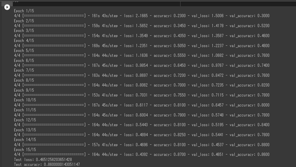

結果としては90%近いのでかなり信憑性の高い判別ができると思います。
5.HTMLとFlaskコードの作成
import os
from flask import Flask, request, redirect, render_template, flash
from werkzeug.utils import secure_filename
from tensorflow.keras.models import Sequential, load_model
from tensorflow.keras.preprocessing import image
from PIL import Image
import numpy as np


# バイクメーカーのクラス
classes = ["ZX10R", "KATANA", "CB1100R", "VMAX", "XL1200"]

# 画像サイズ
image_size = 150  # 画像サイズを整数値に変更
  # 学習に使用した画像サイズに合わせて設定

UPLOAD_FOLDER = "uploads"
ALLOWED_EXTENSIONS = {"png", "jpg", "jpeg", "gif"}

app = Flask(__name__)

def allowed_file(filename):
    return "." in filename and filename.rsplit(".", 1)[1].lower() in ALLOWED_EXTENSIONS

model = load_model("./model.h5")  # 学習済みモデルのファイル名を指定

@app.route('/', methods=['GET', 'POST'])
def upload_file():
    if request.method == 'POST':
        if 'file' not in request.files:
            flash('ファイルがありません')
            return redirect(request.url)
        file = request.files['file']
        if file.filename == '':
            flash('ファイルがありません')
            return redirect(request.url)
        if file and allowed_file(file.filename):
            filename = secure_filename(file.filename)
            file.save(os.path.join(UPLOAD_FOLDER, filename))
            filepath = os.path.join(UPLOAD_FOLDER, filename)

            # 受け取った画像を読み込み、予測モデルの入力サイズにリサイズ
            img = image.load_img(filepath, target_size=(224, 224))
            img = image.img_to_array(img)
            img = img / 255.0  # 画像の正規化
            data = np.array([img])

            # 以下は変更のない既存のコード
            result = model.predict(data)[0]
            predicted = result.argmax()
            pred_answer = "このバイクは " + classes[predicted] + " です"

            return render_template("index.html", answer=pred_answer)

    return render_template("index.html", answer="")

if __name__ == "__main__":
    port = int(os.environ.get('PORT', 8080))
    app.run(host ='0.0.0.0',port = port)
6.アプリの動作確認

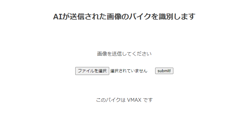

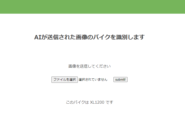
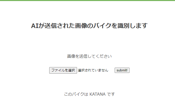
ちゃんと車両の判別が、しっかりできています。
7.改善点
画像の形式の違いなどで読み込めない画像などがありサンプルデータが偏ってしまい学習数値が思ったように上がらず色々と調べるうちに画像ファイルの形式がバラバラだということに気づき統一することにより問題は解消された。
batchsizeを36でやっていたが調べてるうちにサンプルと同じ数にするといい結果がでるという記事を見たので50でやってみるとすんなり正答率が高まった。
8.結果
結果としては90%に少し足りないくらいまでのところまで数値はあがった。
もう少し時間があれば100%に近づけれたかなと思う。
未経験aidemyの機械学習マスター講座を受講してみて、pythonの基礎からディープラーニングやAIについてなど色々なことを学べました。slackで簡単に質問もでき、少し深いことを質問したい時はグーグルミートでメンターの方と顔を合わせて質問したりと環境的には非常によかったです。
思いのほか学習に時間を使えず自分が思っていたレベルまで到達出来なかったのは心残りです。
今後も学習は続けていき、本来の目的であった画像の判別でメーカーを当てるというものを作成したいと思います。
最後にAidemyの方々に初心者の私にも親切にサポートいただきましたこと感謝申し上げます。