環境
- PC:windows10
- 言語 :python 3.6.7
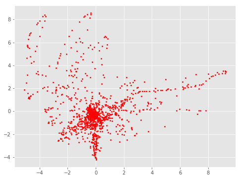
現実のデータは汚い
重複の多いデータを間引きたいときがあります.
重複が多いと処理も増えるし,機械学習では重複サンプルの寄与が大きくなりすぎて問題になることもあります.
下図は,過剰に重複があるようなデータです.
間引き処理後
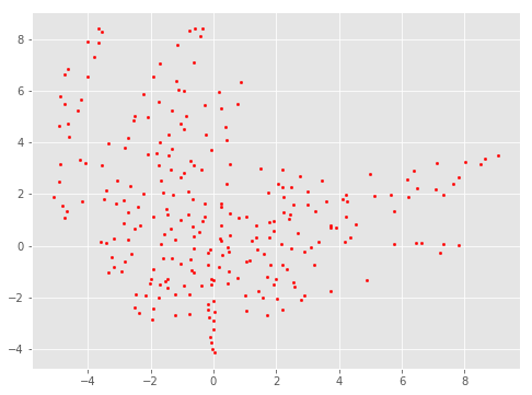
この記事では,代表サンプルだけを残し,誤差を許容しながら高速に重複データを間引く処理を紹介します.
スライシングとかダウンサンプリングはダメなの?
ランダムにサンプリングしたり,サンプリングレートを下げるのも有効ですが,「重複しているデータだけを間引いて,それ以外は全部保持したい」場合,それらの手法は有効ではないことがあります.
ここで紹介する手法は,そのような場合に有効なものです.
紹介する方法はどのくらい高速か?
一般的なノートPCのCPUを用いて,
100次元1万サンプルを対象にして0.05sec,
1000次元10万サンプルを対象にして8secほどで処理が完了します.
密度情報が失われるのでは?
大丈夫です.密度情報も残しながら間引きます.
どうやるか?
次のようなnumpy配列を適切に間引きたいとします.1行が1個のサンプルに対応しているとします.
X = np.array([[1.   , 1.   ],
              [1.001, 1.001],
              [2.   , 2.   ],
              [2.002, 2.002],
              [3.   , 3.   ],
              [3.003, 3.003],
              [4.   , 4.   ],
              [4.004, 4.004],
              [5.   , 5.   ],
              [5.005, 5.005]])
ここで,[1. , 1. ]と[1.001, 1.001]はほとんど同じと見なせるので,どちらか間引きたいところです.
NumPyには,全く同じ配列を間引くuniqueメソッドが用意されていますが,これは全く同じ配列しか間引けないため,上のように誤差を許容して間引きたい場合には工夫が必要です.
そこで,四捨五入するためのroundメソッドと組み合わせます.
import numpy as np

def thin_out(X):
    X_rounded = np.round(X, decimals=0)
    return np.unique(X_rounded, axis=0)
これに先ほどの配列を代入すると
thin_out(X)
array([[1., 1.],
       [2., 2.],
       [3., 3.],
       [4., 4.],
       [5., 5.]])
このように,誤差を許容して間引くことができます.
使い勝手は微妙じゃないか?
このままでは正直使いづらいです.重複を間引く基準が,何桁目を四捨五入するかに依存しているからです.
そこで,間引くときの細かさをもっと柔軟に変えられるようにします.
クラス版
import numpy as np
from sklearn.preprocessing import MinMaxScaler

def np_unique_with_tolerance(ar, decimals, axis):
    """誤差を許容しつつ,重複を排除した配列を生成する"""
    # 四捨五入する
    ar_rounded = np.round(ar, decimals=decimals)
    # 重複を削除し,代表サンプルのインデックスなどの情報を取得する
    ar_unique, index, inverse, counts = np.unique(ar_rounded, axis=axis, return_index=True, return_inverse=True, return_counts=True)
    return index, inverse, counts

class ThinningManager:
    """間引き処理用クラス"""
    def __init__(self, division_num: int = 100):
        self.X = None  # 間引き後のサンプル全体
        self.index = None  # 代表サンプルのインデックス全体
        self.inverse = None  # 元のサンプルがどの代表サンプルに属するか
        self.counts = None  # 代表サンプルがいくつのサンプルを代表しているか
        self.scaler = MinMaxScaler(feature_range=(0,division_num))

    def fit(self, X: "np.2darray"):
        """間引き処理を実行する"""
        # min max normalizationを実行する
        X_scaled = self.scaler.fit_transform(X)
        # 間引き処理を実行する
        index, inverse, counts = np_unique_with_tolerance(X_scaled, decimals=0, axis=0)
        # 間引き後のデータを登録する
        self.X = X[index]
        self.index = index
        self.inverse = inverse
        self.counts = counts

    def get_X(self):
        """間引き後のデータを取得する"""
        return self.X
division_numで間引きの粒度を調整できるようになっています.
division_numが0に近いほど荒く,大きいほど細かく代表サンプルを残します.
ボストン住宅価格データセットを間引いてみる
とりあえずロード
from sklearn.datasets import load_boston

boston = load_boston()
data = boston["data"]
print(data.shape)
(506, 13)
506個のサンプルが含まれています.
標準化して,間引き処理の効果のわかりやすさのために2次元まで落とします.
import sklearn.decomposition
from sklearn.preprocessing import StandardScaler

ss = StandardScaler()
pca = sklearn.decomposition.PCA(n_components=2)

data_after_ss = ss.fit_transform(data)
data_after_pca = pca.fit_transform(data_after_ss)
print(data_after_pca)
(506, 2)
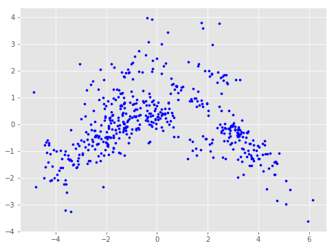
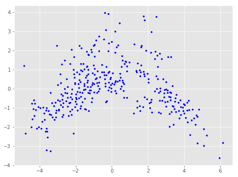
散布図を描いてみます.
import matplotlib.pyplot as plt

X = data_after_pca[:,0]
Y = data_after_pca[:,1]
fig = plt.figure(figsize=(8,6))
plt.scatter(X,Y, s=10, c="blue")
plt.show()
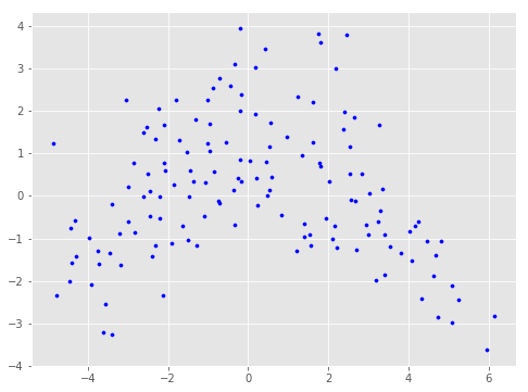
division_num=50で間引く
tm = ThinningManager(division_num=50)
tm.fit(data_after_pca)
data_after_thinning = tm.get_X()
print(data_after_thinning.shape)
(339, 2)
339個まで減りました.散布図も若干まばらになっています.
division_num=20で間引く
もっと荒くしてみます.
tm = ThinningManager(division_num=20)
tm.fit(data_after_pca)
data_after_thinning = tm.get_X()
print(data_after_thinning.shape)
(143, 2)
143個まで減りました.
できるだけ細かくサンプルを残したいときは,division_numを大きくしてください.
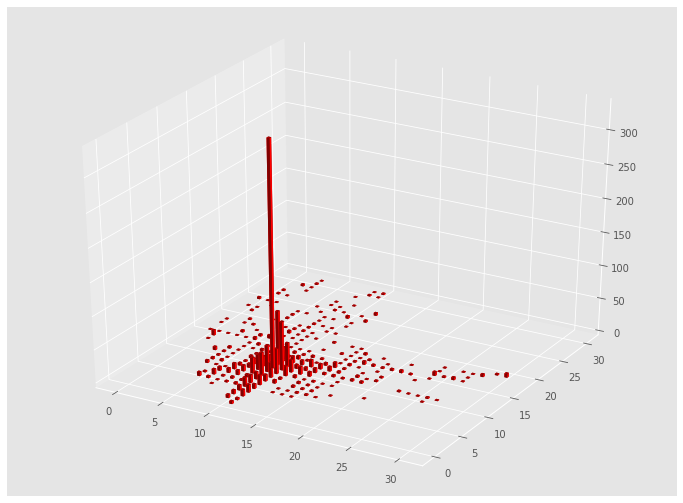
重複個数も表示してみる
from mpl_toolkits.mplot3d import Axes3D

fig = plt.figure(figsize=(12, 9))
ax1 = fig.add_subplot(111, projection='3d')

top = tm.counts
bottom = np.zeros_like(top)
width = depth = 0.1

ax1.bar3d(X, Y, bottom, width, depth, top, shade=True, color="royalblue")
plt.show()
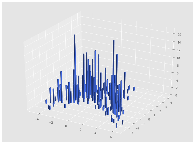
このように,おおまかな密度も見ることができます.(正確に密度を見るならヒストグラムなどの道具を使うべきです)
処理速度
jupyter notebookの%timeitコマンドを使って処理時間を測ってみます.
tm = ThinningManager(division_num=50)
%timeit tm.fit(data_after_pca)
420 µs ± 6.18 µs per loop (mean ± std. dev. of 7 runs, 1000 loops each)
一般的なCPUでも,わずか420µsで完了しました.使用したCPUはCore i7-8550Uです.
極端に高次元かつ多サンプルの場合は?
1000次元1000万サンプルくらいまでは現実的な時間で処理が完了しますが,それ以上に多くのデータを扱いたい場合はメモリ管理が必要になり,PCAなどの次元削減やミニバッチ処理といったテクニックが重要になってきます.
記事は以上です.機会があればご活用ください.