sklearnの回帰モデルを片っ端から試す

はじめに

sklearnの回帰モデルを28種類試し，精度のグラフを生成します．

機械学習モデルを大量に試すツールとしてはAutoML系や, 最近ではPyCaretのように素晴らしく便利なものが巷に溢れていますが，自前でモデルを用意したいことがあったので，備忘録を残します．

環境

• Python 3.6.10
• scikit-learn 0.22.0

コード

回帰モデルのインポート

必要なモデルをインポートし，全ての回帰モデルのインスタンスをまとめます．

from sklearn.linear_model import LinearRegression, Ridge, Lasso, ElasticNet, SGDRegressor
from sklearn.linear_model import PassiveAggressiveRegressor, ARDRegression, RidgeCV
from sklearn.linear_model import TheilSenRegressor, RANSACRegressor, HuberRegressor
from sklearn.neural_network import MLPRegressor
from sklearn.svm import SVR, LinearSVR
from sklearn.neighbors import KNeighborsRegressor
from sklearn.gaussian_process import GaussianProcessRegressor
from sklearn.tree import DecisionTreeRegressor
from sklearn.experimental import enable_hist_gradient_boosting
from sklearn.ensemble import RandomForestRegressor, AdaBoostRegressor, ExtraTreesRegressor, HistGradientBoostingRegressor
from sklearn.ensemble import BaggingRegressor, GradientBoostingRegressor, VotingRegressor, StackingRegressor
from sklearn.preprocessing import PolynomialFeatures
from sklearn.pipeline import Pipeline
from sklearn.cross_decomposition import PLSRegression

reg_dict = {"LinearRegression": LinearRegression(),
            "Ridge": Ridge(),
            "Lasso": Lasso(),
            "ElasticNet": ElasticNet(), 
            "Polynomial_deg2": Pipeline([('poly', PolynomialFeatures(degree=2)),('linear', LinearRegression())]),
            "Polynomial_deg3": Pipeline([('poly', PolynomialFeatures(degree=3)),('linear', LinearRegression())]),
            "Polynomial_deg4": Pipeline([('poly', PolynomialFeatures(degree=4)),('linear', LinearRegression())]),
            "Polynomial_deg5": Pipeline([('poly', PolynomialFeatures(degree=5)),('linear', LinearRegression())]),
            "KNeighborsRegressor": KNeighborsRegressor(n_neighbors=3),
            "DecisionTreeRegressor": DecisionTreeRegressor(),
            "RandomForestRegressor": RandomForestRegressor(),
            "SVR": SVR(kernel='rbf', C=1e3, gamma=0.1, epsilon=0.1),
            "GaussianProcessRegressor": GaussianProcessRegressor(),
            "SGDRegressor": SGDRegressor(),
            "MLPRegressor": MLPRegressor(hidden_layer_sizes=(10,10), max_iter=100, early_stopping=True, n_iter_no_change=5),
            "ExtraTreesRegressor": ExtraTreesRegressor(n_estimators=100), 
            "PLSRegression": PLSRegression(n_components=10),
            "PassiveAggressiveRegressor": PassiveAggressiveRegressor(max_iter=100, tol=1e-3),
            "TheilSenRegressor": TheilSenRegressor(random_state=0),
            "RANSACRegressor": RANSACRegressor(random_state=0),
            "HistGradientBoostingRegressor": HistGradientBoostingRegressor(),
            "AdaBoostRegressor": AdaBoostRegressor(random_state=0, n_estimators=100),
            "BaggingRegressor": BaggingRegressor(base_estimator=SVR(), n_estimators=10),
            "GradientBoostingRegressor": GradientBoostingRegressor(random_state=0),
            "VotingRegressor": VotingRegressor([('lr', LinearRegression()), ('rf', RandomForestRegressor(n_estimators=10))]),
            "StackingRegressor": StackingRegressor(estimators=[('lr', RidgeCV()), ('svr', LinearSVR())], final_estimator=RandomForestRegressor(n_estimators=10)),
            "ARDRegression": ARDRegression(),
            "HuberRegressor": HuberRegressor(),
                    }

注意１　各回帰モデルの引数はかなりテキトーで，上のコードは用例に過ぎません．使用する際にはデータに応じた適切な値にしたり，グリッドサーチのようなハイパーパラメータ最適化と組み合わせることを強く推奨します．

注意２　Polynomial_deg2～5は2～5次関数による回帰です．他のモデルの解説はsklearn公式を参照してください．

回帰用データの生成と，学習

sklearnのmake_regressionを使って，回帰のためのデータを生成します．

さらに，全モデルを10回ずつ学習・推論させて，精度（ここではMAPEを使用）の良い順にソートします．

from sklearn.model_selection import train_test_split
import random
from sklearn.datasets import make_regression
import numpy as np

def mean_absolute_percentage_error(y_true, y_pred):
    """MAPE"""
    return np.mean(np.abs((y_true - y_pred) / y_true)) * 100

test_size = 0.3  # 分割比率
N_trials = 10  # 試行回数

# 回帰対象のデータを生成
x, y = make_regression(random_state=12, 
                       n_samples=100, 
                       n_features=10,
                       n_informative=4,
                       noise=10.0,
                       bias=0.0)

mape_dict = {reg_name:[] for reg_name in reg_dict.keys()}  # 精度の格納庫

for i in range(N_trials):
    print(f"Trial {i+1}")
    random_state = random.randint(0, 1000)
    x_train, x_test, y_train, y_test = train_test_split(x, y, test_size=test_size, random_state=random_state)

    for reg_name, reg in reg_dict.items():
        reg.fit(x_train,y_train)
        y_pred = reg.predict(x_test)
        mape = mean_absolute_percentage_error(y_test, y_pred)  # MAPEを算出
        mape_dict[reg_name].append(mape)  # 格納

# MAPEの平均値でソート
mape_dict_sorted = {key: value for key, value in reversed(sorted(mape_dict.items(), key=lambda x:np.mean(x[1])))}

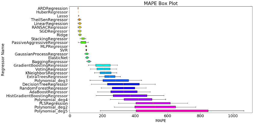
結果のプロット

上では全モデルに対してMAPEを10回ずつ計測し，MAPEの平均値でソートしました．

機械学習モデルの良し悪しを判断する際には，精度の平均値のほかに散らばり具合（分散のような指標）も見ておきたいところです．

そこで，箱ひげ図を描画します．

MAPEは小さいほど良いので，図中だと上のモデルほど良く，さらに箱ひげが小さいほど安定したモデルと解釈できそうです．

import matplotlib.pyplot as plt
import matplotlib.cm as cm
from matplotlib.colors import Normalize

plt.rcParams["font.size"] = 18  # フォントサイズを大きくする
scalarMap = cm.ScalarMappable(norm=Normalize(vmin=0, vmax=len(mape_dict)), cmap=plt.get_cmap('gist_rainbow_r'))

plt.figure(figsize=(15,9))
box=plt.boxplot(mape_dict_sorted.values(), vert=False, patch_artist=True,labels=mape_dict_sorted.keys())
for i, patch in enumerate(box['boxes']):
    patch.set_facecolor(scalarMap.to_rgba(i))
plt.title("MAPE Box Plot")
plt.xlabel("MAPE")
plt.ylabel("Regressor Name")
plt.show()