
title: 'Nobody Checks a Mathematical Picture, Because It Already Looks Right — A PoC Series Where the Theorem Is the Test'
tags:
- Python
- NumPy
- 数学
- アルゴリズム
- 画像処理
public_private: false
public_id: dc100e7ea90e9575c40b
Language: 日本語 · English
Nobody Checks a Mathematical Picture, Because It Already Looks Right — A PoC Series Where the Theorem Is the Test

↑ As the arms go 1 → 4 → 16 → 90 → 600 → 4000, the picture gives itself away. How close it gets at each stage is known before anything is drawn.
About the figures: every figure from the seven runs this article covers is shown below (86 of them). All 151 runs and 1165 figures, including those outside this series, are laid out in the metrology museum; the files themselves are here.
About this series
Domain colouring. Newton basins. The Mandelbrot set. Apollonian gaskets. Phyllotactic spirals. Flow around an aerofoil. Mathematical pictures look right. And things that look right never get checked.
If the implementation is slightly wrong, the picture is still beautiful. The hues still wind, the boundary is still fractal, the circles still pack. The error does not show up in the picture — that is what makes this subject hard to write about honestly.
So the bar for adding a drawing routine was cut down to two questions:
(i) Is there a theorem that can act as the gate, or (ii) does an existing, independent implementation supply the truth?
If neither, don't write it. Checking a formula against itself is forbidden.
Each instalment is one drawing built to that bar, and each one ships with a scorecard. The code is in fullseye, and every figure is the output of the script itself.
Where the series is
| # | What gets drawn | The gate (where the truth comes from) |
|---|---|---|
| 1 | A photograph as one line, drawn by rotating circles | Parseval's identity / the minimum spanning tree as a lower bound |
| 2 | The complex plane as an area, not a curve | The argument principle / Cayley 1879 / the closed form of the main cardioid |
| 3 | Theorems that happen to be pictures | Descartes' circle theorem / Farey neighbours / Euler's formula / Moran's equation |
| 4 | One beat — a two-slit fringe and a print moiré are the same mathematics | Closed-form eigenvalues / zeros of Bessel functions / the grating equation / a predicted moiré period |
| 5 | What a picture cannot check — dynamical systems and minimal surfaces | The matrix exponential / the trace identity / exact bifurcation points / the definition H ≡ 0 |
| 6 | Making pictures that lie to the eye, then grading the measurement | Lucas' theorem / Descartes' circle theorem / div(curl ψ) ≡ 0 / mass conservation |
| 7 | Auditing the instrument — where a caliper fails, and why | Ground truth guaranteed by the generator / the fit residual / a declared expected width / the definition of an edge |
1. A photograph as one line, drawn by rotating circles
Recipe
photo → stipple → one closed line → resample to equal arc length → Fourier coefficients → redraw with rotating circles
Tone becomes point density (weighted Lloyd), a tour visits every point exactly once and returns (TSP), the tour is resampled to equal arc length and expanded as a complex Fourier series. The Fourier series of a closed curve is a sum of rotating arms, so it becomes a chain of pendulums with nothing added.
The lineage is TSP art (Kaplan & Bosch 2005). A tour being closed is exactly the condition for putting it on a Fourier series, so the two ideas were already made for each other.
| Term | In plain words |
|---|---|
| Stippling | Put more dots where it is dark; density carries the tone |
| Weighted Lloyd | Repeatedly move each point to the centroid of its own territory |
| Minimum spanning tree (MST) | The shortest tree joining all points. A closed tour can never be shorter than this |
| Parseval's identity | "Total energy = sum of squared coefficients". The truncation error can be computed in advance |
Gates and scores
Measured on Hokusai's Great Wave (202×300 px) with 9,000 points. The truths used are only of three kinds — a lower bound, a control group, and a closed form. No special apparatus.
| Claim | Measured | Where the truth comes from | Control |
|---|---|---|---|
| Density follows tone | correlation 0.9946 | banded darkness of a ramp image | evenly spread on a uniform image (cv 0.13 vs 0.37) |
| Tour quality | 1.146 × MST | a closed tour cannot beat the MST | joining in coordinate order: 41.4 × |
| Tone reproduction | correlation 0.984 | direct comparison with the target | the same number of random lines: +0.013 |
| Pen width | 0.900 px | ink ≈ length × width / area | 0.890 × of target; the missing 11 % is overlap |
| Number of circles | 99.0 % at K=64 | Parseval's identity | prediction vs measurement differ by 7e-15 px |
| On paper | 15.57 m / 8.6 min | converted to G-code and measured | — |

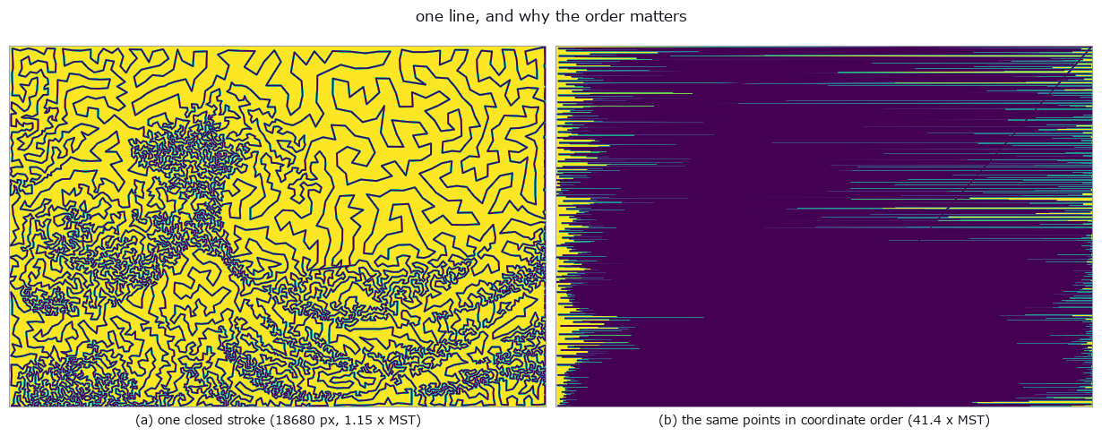
↑ Left: the single stroke (1.146 × MST). Right: the same points joined in coordinate order (41.4 ×). Same points — the difference is entirely in the joining.
★ Where you will get it wrong
Four traps sit on this path. None of them raises an exception, and the picture looks plausible in every case, so you only find them by writing the test.
1. High correlation does not mean density is proportional to darkness
Measure "density follows tone" by correlation and you get above 0.99. But correlation only sees monotonicity.
Weighted Lloyd produces a centroidal Voronoi tessellation, and by Gersho's conjecture the optimal point density goes like √ρ in the weight ρ (ρ^(d/(d+2)) in d dimensions). Pass the weight straight through and only half of your tone range reaches the paper.
Measure the exponent directly (the slope of log density against log darkness) and it is 0.61. A correlation of 0.9946 and an exponent of 0.61 are not in conflict — the relation is monotone, so the correlation is high.
If you want proportionality to tone, pass the square of the weight. Measured, the exponent rises to 0.77 (it will not reach 1 because of the floor and the finite point count).
2. The line has already got shorter before it reaches the Fourier series
When the tour is resampled to equal arc length, a sample spacing coarser than the segments cuts the corners and shortens the line itself. Information is lost before the transform, so any later "the prediction was right" rests on nothing.
On a tour whose segments are 2.08 px on average and 1.57 px at the median:
| Resample points | Spacing | Length retained | Shortest representable period |
|---|---|---|---|
| 16,384 | 1.140 px | 0.935 | 2.28 px |
| 32,768 | 0.570 px | 0.967 | 1.14 px |
| 65,536 | 0.285 px | 0.984 | 0.57 px |
At 1.14 px the dense regions are unresolved and the line shrinks by 6.5 %. The error falls cleanly as 1/N, so the rule of thumb is to raise N until the spacing is below the median segment length.
3. An even point count double-counts a Fourier coefficient
Taking complex coefficients over k = −N/2 … +N/2, an even N makes the two ends the same coefficient. Add both and Parseval's identity breaks (1.17e-01 at N=8, 7.5e-03 at N=512).
The nasty part is that a highly symmetric shape hides it: check on the outline of a square and the highest-frequency coefficient happens to be near zero, so it passes. Sweep N over 8, 9, 16, 17, 64, 255, 256 and pin down both the coefficient count and Parseval.
4. Pen width is not tuned, it is solved
While the lines do not overlap, ink ≈ length × width / area holds, so you can solve for the pen width from the target darkness.
Two caveats. First, stamping the line with integer-pixel discs makes the width a staircase — 0.5 / 1.0 / 1.5 px give the same picture. Fill by coverage and it becomes a continuous knob.
Second, even the solved width undershoots. Measured ink was 0.890 × the target. A union is smaller than a sum, so the measurement is always below the prediction, and that 11 % gap is the amount of overlap. Reading it as a measurement of overlap rather than as an error is the point.
What it is bad at
It is bad at ink-line drawings. A centroidal Voronoi tessellation always fills the whole frame, so in a picture where only a few per cent of pixels are dark, most points land on white. On Chōjū-giga (5.5 % dark pixels) the original is unreadable. Line art should be thinned and traced, which is a different tool.
No edge-following term was added. With one, the fraction of line running near an edge rises from 0.421 to 0.530, but the tone correlation drops from 0.911 to 0.772 and the density contrast from 6.5 to 2.4 — both get worse. In this picture the edges are already dark, so raising the tone contrast improves both (the edge area fraction is 0.235, so 0.235 of the line would sit on edges by chance; tone alone gives 0.475, already twice that).
Run it
pip install -U fullseye
py -3.11 examples/poc_one_stroke_epicycles.py \
    --image my_photo.jpg --points 12000 --out out/mine
Point count scales as pixels × points. Start at --points 3000 to see the shape, then raise it.
import fullseye as fs

img  = fs.read_image("photo.png")
pts  = fs.ledger.stipple_points_from_image(img, 9000, gamma=1.6)  # dots where it is dark
tour = fs.ledger.stroke_tour_closed(pts)                           # one closed line
err  = fs.ledger.stroke_tone_error(img, tour)                      # what was preserved, as a number
print(err["corr"], err["length_px"])
This run produced 9 figures in total - see them all
The rest of this run's figures
The remaining 6 figures from the same run. Captions are cut to their first sentence; the detailed reading belongs to the figures above.

↑ Lloyd's energy sum w|x-c(x)|^2 never goes up — that is a property of the algorithm that can be checked exactly, which is why it is the gate rather than the look…

↑ the tone of a line drawing exists at a scale coarser than the line, so both pictures are compared after a Gaussian of sigma 6 px: correlation 0.984 against +0.0…

↑ while the strokes do not overlap the ink fraction is length x width / area, so the width that reproduces the mean tone is solved in closed form (0.90 px here)

↑ Parseval makes this a prediction, not a measurement: the squared error of the order-K reconstruction equals the energy of the coefficients above K, exactly

↑ every row is measured by an operator in this run; the harmonic rows are predicted in closed form before the drawing is made

↑ Parseval: the error above is the energy that was left out, exactly
2. The complex plane as an area, not a curve
Recipe
a rational f(z) → evaluate over an area → domain colouring / basins / escape time → score against a truth outside the picture
Visualising complex analysis needs different tools on a curve (integrals, winding numbers, Laurent coefficients, conformal maps) and over an area (the value field, domain colouring, basins). This instalment is the second kind.

↑ None of these can be checked by looking. Every score below comes from outside the picture.
Gates and scores
| Claim | Measured | Value | Where the truth comes from |
|---|---|---|---|
| Argument principle | winding number | +3 / +1 / −2 | the existing cplx_winding_number (zeros outside the window count 0 — the control) |
| The order is readable from the picture | hue winding, from the pixel RGB alone | 1 / 2 / 3 / −2 | the argument principle |
Basins of z²−1
|
agreement with the exact solution | all 262,144 pixels, 0 unconverged | Cayley 1879 (two half-planes) |
| Basins of a cubic | boundary pixels on the same grid | 1,026 → 13,348 (13 ×) | the case Cayley could not solve |
| Main cardioid | pixels declared interior without iterating | 0 counterexamples, covering 90.1 % | a closed form (the fact that it is a lower bound is also a number) |
| Flow around the aerofoil | Cauchy–Riemann residual | 2.06e-04 | controls: random 1.04, conjugated 2.000 |
| Circulation is path-independent | outer / inner contour | −3.0263 / −3.0263 | Cauchy's integral theorem |
| The Kutta condition | trailing-edge speed | 22.9 → 22,020 with zero circulation | the control diverges |
A bonus that was not in the plan: the ratio of the lift coefficient to thin-aerofoil theory is exactly a/b — the radius of the circle over the distance to the singularity of the map — independent of angle of attack and of speed. The measured deviation is 2.2e-16, and letting the thickness go to zero recovers thin-aerofoil theory. The whole effect of thickness collapses into one number.
★ Where you will get it wrong
An existing op looked broken, but the caller was. cplx_cr_residual returned 0.95 on a holomorphic field and 1.04 on noise, which reads as "it does not discriminate". Then the docstring: "rows run in the direction of increasing imaginary part." This grid was in image order (rows going down), so the op was correctly measuring the conjugate field.
Breaking a convention does not raise an exception. It returns a different quantity, plausibly. So the discrepancy was turned into a gate rather than left as a trap — the same test now asserts both "2 when passed as is" and "≈ 0 when flipped".
(Exactly 2 only appears where the central difference is exact, i.e. polynomials of degree ≤ 2. On a general holomorphic field it comes out slightly under, by the same rounding floor — measured 1.999951.)
What it is bad at
Escape time is cut off at an iteration limit, so near the boundary there is always a "still undecided" band that grows as you raise the limit. The closed-form interior test is a lower bound and does not cover the whole interior (90.1 % measured). Domain colouring gives you the order of a zero but not its position — that is the job of the op that counts winding numbers.
The first line to run
import fullseye as fs

z = fs.cplx_plane_grid((-2.0, 1.0), (-1.5, 1.5), (512, 512))
basins = fs.cplx_newton_basins((1.0, 0.0, -1.0), shape=(512, 512))  # z^2 - 1
print("unconverged:", int((basins < 0).sum()))          # Cayley's exact solution says 0
This run produced 10 figures in total - see them all
The rest of this run's figures
The remaining 9 figures from the same run. Captions are cut to their first sentence; the detailed reading belongs to the figures above.

↑ 有理関数 (z−z₁)(z−z₂)/(z−p) の位相彩色。

↑ ★絵が定理を証明する側に回る。

↑ 2 次の境界は虚軸 1 本(513 画素の格子で 1026)。

↑ ★★右の明るい部分は反復せずに内側と分かる領域 —— 固定点 z = (1−√(1−4c))/2 が吸引的(|2z*| < 1)なら軌道は決して 脱出しない、という閉形式。*

↑ z → z² + c は |z| を 2 乗するだけなので、c = 0 では「|z| < 1 は 0 へ、|z| > 1 は無限へ」が厳密に言える。

↑ 迎角 8 度のジューコフスキー翼まわりの非粘性流。

↑ 後縁は写像の特異点(dz/dζ = 0)なので、循環が正しくないと1/√距離 で発散する。

↑ ★CL = 2π(a/b)sin(α+β)。

↑ どの行も「使った式」ではない真値で採点している: 既存 op (cplx_winding_number / cplx_cr_residual)、Cayley の定理、閉形式の内部判定、c=0 のジュリア集合、クッタ条件の対照群、薄翼理論との比。
3. Theorems that happen to be pictures
Recipe
a curvature quadruple / Farey denominators / the golden angle / IFS maps / a curve order → a picture
                                   ↓
              then check from the theorem's side, without looking at the picture
Apollonian gaskets, Ford circles, geodesic domes, phyllotactic spirals, IFS attractors, space-filling curves. A slightly wrong implementation still packs circles, still spirals, and still looks fractal.

Gates and scores
| Claim | Measured | Value | Where the truth comes from |
|---|---|---|---|
| Descartes' circle theorem | relative error of (Σk)² − 2Σk²
|
below 1e-13 (all tangent quadruples of the 164 circles at depth 4) | the theorem |
| Integral packing | deviation of curvatures from integers | 0 | Lagarias–Mallows–Wilks |
| Farey adjacency | disagreements between tangency and |ps − qr| = 1
|
0 of 1,081 pairs (47 circles up to denominator 12) | an identity in integers |
| Ford circle count | |F_n| |
matches |
1 + Σφ(k) (Euler's totient) |
| Geodesic dome | degree-5 vertices | exactly 12 at f = 1, 2, 3, 4, 6 | V − E + F = 2 |
| Phyllotaxis | peaks of the index gap that are Fibonacci | golden angle 7/7; 137.0° 2/7; 90° 2/7 | the Fibonacci numbers |
| IFS dimension | similarity vs box counting | 1.5850 (closed form) / 1.6164 (boxes) | Moran's equation Σrᵢᵈ = 1
|
| Space-filling curve | visits 4ⁿ cells once, unit steps | holds for all four kinds | being a permutation |
| Locality | mean distance at k=32 | Hilbert 6.38 / raster 16.07 |
√32 = 5.66 / 32
|
★ This is the point of the instalment. The dome's vertex degrees are counted by a different, existing implementation (conngraph.graph_degree_table). Counting them yourself and agreeing with yourself proves nothing.
Descartes' theorem is set up the same way. Generation uses the reflection k' = 2(k₁+k₂+k₃) − k₄, so tangency is re-discovered from distances before being fed to the theorem — which makes the centre calculation part of what is being tested.
Then the integral packing. A gasket seeded with (−1, 2, 2, 3) has integer curvatures for ever. Drift even slightly and the integers break — an error a picture can never show.
★ Where you will get it wrong
Two defects were found in the tests themselves.
-
pytest.raises(match="similarit")always passes, because it matches the op's own nameifs_similarity_dimension. On top of that the preset name was wrong ("fern"; the correct one is"barnsley_fern"), so the test was watching an unknown-preset rejection and calling it a pass. Checking that something was rejected without checking why gets you this. - Declaring the output type as
pointstripped the type-contract gate.pointsis (N,3) in three dimensions; a list of 2-D points ispairs. The names are close enough to swap by accident.
And a figure exposed a blind spot in the numeric tests. The dome figure rasterised one triangle at a time, so each call normalised to its own bounding box and the result was "a pile of lines each stretched across the whole frame". All 20 numeric checks passed — there was no way to notice before opening the picture.
What it is bad at
The Apollonian gasket grows as a power of 3 in depth (118,100 circles at depth 10). Ford circles shrink as the square of the denominator, so past denominator 30 most of them are under a pixel. The IFS chaos game plots points, so fine gaps need more points to fill (which is why the box-counting dimension comes out above the closed form). Moran's equation applies only to similarities — Barnsley's fern, affine but not similar, is refused.
The first line to run
import fullseye as fs

t = fs.ledger.circle_packing_apollonian(curvatures=(-1, 2, 2, 3), depth=4)
print(len(t["x"]), "circles / still integral:",
      abs(t["curvature"] - t["curvature"].round()).max())

pts  = fs.ledger.phyllotaxis_pattern(n_points=800)
gaps = fs.ledger.neighbour_index_gaps(pts, k=6)
print("peaks of the index gap:", gaps.argsort()[::-1][:5])   # 8, 13, 21, ... at the golden angle
This run produced 11 figures in total - see them all
The rest of this run's figures
The remaining 10 figures from the same run. Captions are cut to their first sentence; the detailed reading belongs to the figures above.

↑ 合計は 2·3^depth + 2。

↑ フォードの円(分母 12 まで、47 円)。

↑ 分割 f を 1, 2, 3, 4, 6 と上げても、次数 5 の頂点はちょうど 12 個から動かない(次数 6 だけが増える)。

↑ オイラーの公式 V − E + F = 2 の帰結。

↑ 3 枚とも螺旋に見える。

↑ 黄金角の山は [34, 55, 89, 21, 13, 8, 144] —— すべてフィボナッチ数。

↑ モランの式 Σrᵢᵈ = 1 は写像の縮小率だけから d を出す。

↑ order 5 で 4^5 = 1,024 点をちょうど 1 回ずつ通り、隣り合う点は必ず距離 1。

↑ ヒルベルトは √k の近くを通り(k=32 で 6.38)、走査線はほぼ k に比例する(16.07)。

↑ どの行も「使った式」ではない真値で採点している: デカルトの円定理、整数充填、|ps − qr| = 1、オイラーの関数の和、オイラーの公式(既存 graph_degree_table が数えた)、フィボナッチ、モランの式と既存 fractal_dimension、置換であること。
4. One beat — a two-slit fringe and a print moiré are the same mathematics
Recipe
membrane eigenmodes / two slits / a diffraction grating      ┐
                                                             ├→ both are "the difference of two frequency vectors"
two superposed halftone screens / engraving / hatching / mosaic ┘
A two-slit fringe and the moiré of two superposed halftone screens live in different textbook chapters. There is only one formula. This instalment checks that one formula from both ends.

↑ The mode shape is signed ([-1, 1]): the phase flips across a nodal line, so calling it an image2d would throw the antinode phase away.
Gates and scores
| Claim | Measured | Value | Where the truth comes from |
|---|---|---|---|
| Rectangular membrane eigenvalues | max difference from π²(m²+n²)
|
0.00e+00 | the closed form, degeneracies included |
| Nodal line count | (m,n)=(3,4), vertical / horizontal | 2 / 3 |
m−1 / n−1 (integers) |
| Circular membrane nodal circles | radii | agree |
the zeros of J₀ over k |
| Two slits | measured period / λD/d
|
0.998–1.003 over four settings | a different op measures it back |
| Diffraction grating | wavelength recovered by an existing op | 550.000000 nm | round trip through grating_wavelengths
|
| Even orders vanish | orders seen | −3, −1, 0, 1, 3 | the Fourier coefficients of a square wave vanish at even harmonics |
| 3rd / 1st intensity ratio | ratio | 0.1140 |
sinc(m/2)² → 1/9 |
| Moiré period | measured / predicted before drawing | 0.948–0.986 | the closed form 1/(2 f sin(Δ/2))
|
| Halftone preserves density | difference through a four-period window | 0.0517 | only the tone scale was discarded |
| Engraving | ink coverage vs w/d
|
0.0000 over four tones | the closed form |
| Hatch direction | offset against a 30° grating | 0.3° | the existing structure_tensor_orientation
|
| Lloyd | energy, iteration 0 → 16 | 2,782,566 → 1,491,442 | the existing stipple_energy measures it (monotone) |
| Cell mean | cells where the minimum is not the mean | 0 (exhaustive) | L2 optimality |
★ Two things I misread, both of them the measurement
The beat is at low frequency. Take the FFT argmax without restricting the search band and you get 16.7 px = the screen's own period 1/f at every angle, which reads as "the prediction is nowhere near".
Hatch strokes are at high frequency. Without a lower cut you pick up not the strokes but the envelope of where the ink went (the same 24 px as the original grating), and the direction looks 90° off.
In both cases the op was right and the defect was in how it was measured. A spectrum always has several peaks, and argmax returns the strongest one, not the one you are looking for. Worse, what comes back is a plausible number — no exception, no NaN, just a different quantity, quietly.
A correction about Chladni figures
The familiar cos·cos − cos·cos is the solution for a membrane, not a plate. A real Chladni plate obeys the biharmonic equation; the sand collects on nodal lines in both pictures, but the frequency ratios do not match. This layer says membrane and scores only against membrane truths (closed-form eigenvalues, Bessel zeros).
And one more: the nodal circles of a circular membrane sit at the zeros of J₀. The zeros of J′₀ are the antinodes. Swap them and a correct op looks broken — which is what happened here, once.
What it is bad at
wave_two_slit is the Fraunhofer far field; the near field and the Fresnel region are a different op's job. Membrane modes are the analytic solutions for a rectangle and a disc only — no arbitrary boundary. wave_fringe_period returns one dominant period, so on an image with several superposed periods it sees only the strongest. The moiré prediction is for two screens of the same kind; three or more plates, and second-order beats from dot-shape differences, are not in it. hatch_field can hold only one direction per pixel, so at crossings and junctions the direction is arbitrary — whether to trust it is reported by the coherence, not the orientation.
The first line to run
import fullseye as fs

# The moiré period is known before you print
p = fs.ledger.halftone_moire_period(lpi_a=60.0, angle_a_deg=45.0,
                                    lpi_b=60.0, angle_b_deg=75.0, pixel_um=25.4)
print("moire period %.2f px / direction %.1f deg" % (p["period_px"][0], p["angle_deg"][0]))

# The fringe period is measured back by a different op from the one that drew it
img = fs.wave_two_slit(wavelength_nm=550.0, slit_sep_um=200.0,
                       distance_mm=200.0, shape=(64, 1024), pixel_um=5.0)
print("measured %.2f px / lambda*D/d = %.2f px"
      % (fs.wave_fringe_period(img), 0.55 * 200e3 / (200.0 * 5.0)))
This run produced 13 figures in total - see them all
The rest of this run's figures
The remaining 12 figures from the same run. Captions are cut to their first sentence; the detailed reading belongs to the figures above.

↑ (m, n) モードの節線は縦 m−1 本・横 n−1 本。

↑ 縞間隔は λD/d。

↑ 重なっていることが主張。

↑ ★デューティ 50 % の矩形格子は偶数次が消える(矩形波のフーリエ係数が偶数調波で 0)。

↑ 新聞の 15° / 45° / 75° は差が 30° で、うなりが最も細かくなる組み合わせ。

↑ ★FFT の探す範囲を切らないとスクリーン自身の山(どの角度でも 16.7 px = 1/f)を拾って「予言と全然合わない」と読める。

↑ 平均絶対差 0.0517。

↑ 被覆率は線幅 / 間隔 = w/d。

↑ 向きは既存 structure_tensor_orientation が決める(この族は構造テンソルを再実装しない)。

↑ Lloyd 反復でセルが等エネルギーに近づく。

↑ 下がり続けることが主張。

↑ どの行も「使った式」ではない真値で採点している: 膜の閉形式とベッセルの零点、λD/d を測り返す別の op、既存 grating_wavelengths との往復、描く前のモアレ予言、w/d の閉形式、既存 structure_tensor_orientation、既存 stipple_energy。
5. What a picture cannot check — dynamical systems and minimal surfaces
Recipe
a named vector field → integrate → sections, exponents, bifurcations, dimensions
exact parametrisations of minimal surfaces → a mesh → let a different op measure the mean curvature
A Lorenz plot is the same butterfly whether the integrator is 1st or 4th order. A minimal surface looks smooth whether or not its mean curvature vanishes. In this instalment, looking gets you nothing at all.

Gates and scores
| Claim | Measured | Value | Where the truth comes from |
|---|---|---|---|
| Order of RK4 | error ratio per halving | 16.0 / 16.0 / 16.0 |
expm(At)x₀ is the exact solution |
| Order of Euler (control) | the same ratio | 2.08 / 2.04 / 2.02 | first order |
| Error at the same step | dt = 0.01 | 2.02e-02 vs 3.33e-10 | orders of magnitude apart |
| The trace identity | Σλ − (−(σ+1+β)) |
2.57e-06 | exact, and independent of how λ was produced |
| Largest Lyapunov exponent | λ₁ | 0.9142 | published 0.906 |
| Conservative control |
Σλ of a harmonic oscillator |
4.87e-15 | 0 |
| First bifurcation | r | 2.999401 | 3 (exact) |
| Second bifurcation | r | 3.449260 | 1+√6 = 3.449490 |
| Feigenbaum δ | (r₂−r₁)/(r₃−r₂) |
4.7485 | 4.6692 |
| Field divergence | existing piv_divergence vs tr(A)
|
under 1e-6 in all four cases | exact for a linear system |
| Field vorticity | existing piv_vorticity vs A₁₀−A₀₁
|
agrees | exact for a linear system |
| Tube mesh | volume / 2π²Rr²
|
0.99667 | the analytic torus |
| Tube mesh | area / 4π²Rr
|
0.99928 | the same |
| Minimal surfaces | median |H| over four families |
0.00002–0.00014 | 0 — the definition itself |
| Controls |
|H| of a unit sphere / cylinder |
1.00004 / 0.50000 | 1.0 / 0.5 (not minimal) |
| Isometric bending | spread in area | 17.6738–17.6756 | unchanged |
| Gyroid | volume fraction at 48³/64³/96³ | 0.499928 / 0.499981 / 0.499991 | 0.5 by the body-centred symmetry |
★ The examiner comes from a different family. ode_vector_field_grid returns a flow2d, so the existing PIV (particle image velocimetry) ops — piv_divergence, piv_vorticity — consume it directly. They know nothing about this family, which makes them an independent examiner for "the field is right". For a linear system the divergence is exactly tr(A) and the vorticity exactly A₁₀ − A₀₁.
For minimal surfaces, the definition is the gate. "Mean curvature H vanishes everywhere" is measured by the existing vertex_curvature — so the claim "this is a minimal surface" is scored by an op that does not know how it was built. The controls come out at 1.00004 (unit sphere) and 0.50000 (unit cylinder), which is also the evidence that the gate is not a pass-through.
Residuals are not hidden
In both cases the cause was located by measurement before anything was written down.
(1) A bifurcation point always looks slightly early. Convergence at a bifurcation is algebraic, not geometric, so a finite burn-in never arrives (δ is biased the same way, 4.7485 against 4.6692, 1.7 %). So the gate is not "the error is small" but "lengthening the burn-in shrinks it by what you left on the table" — 2,000 → 20,000 shrinks it 10.9 ×. That, not the size of the error, is the evidence that the residual is the measurement and not the map.
(2) The correlation-dimension bias was not the sample count. A circle gives 1.0061 and a Cantor set 0.6408 (true value log2/log3 = 0.6309), but a filled square gives 1.8789 against a true value of 2. The first suspect — too few points — was wrong: 400 → 1,500 → 3,000 points gives 1.8825 / 1.8789 / 1.8709, if anything going down.
The cause is the radius window over which the power law is read. The default is the 1st–25th percentile of pair distances, and on a bounded set the upper end runs into the boundary, where the correlation sum saturates and flattens the slope. Narrow the window towards small r and the estimate walks to 1.887 → 1.947 → 2.050.
"Finite sample" and "numerical error" fit anything, which is exactly why writing one stops the investigation. An explanation that fits and an explanation that is right are different things, and only the right one tells you which knob fixes it. Here it was
r_lo/r_hi, notmax_points.
The gyroid is treated the same way. At level = 0 the field is odd under the body-centred inversion, so the volume fraction is exactly 1/2 by symmetry, independent of the grid. But Schoen's gyroid has H = 0, and the nodal approximation keeps a residual (|H| over the principal-curvature scale = 0.1250). It is a scaffold and a picture, not a claim of minimality.
★ Where you will get it wrong
A function whose return type depends on an argument cannot go in a typed ledger. gyroid_isosurface(..., thickness=...) returned a voxel volume with thickness and a mesh without it, but only one output type can be declared — so either declaration is a lie. It was split into two ops.
Splitting it paid off: the solid form dropped its scikit-image dependency and now runs on bare numpy.
One more. ode_vector_field_grid first returned (H, W, 2) and was caught by the type checker. That layout reads more naturally, but flow2d is an existing type with an existing predicate and existing consumers, so returning the transpose is a type lie. Matching the existing vocabulary beat readability — and as a result ten existing ops downstream connected for free.
What it is bad at
A system is named, or given as coefficients; callable is not accepted — a typed ledger registers inputs by type, so a function cannot be one. This is not a door for arbitrary ODEs. Lyapunov exponents cover only the systems whose tangent flow is available; estimation from a delay embedding is not in it. The orbit diagram is for 1-D maps only. For the correlation dimension, state the radius window when the answer matters (the default window reads low on a bounded set, as above). Minimal surfaces are the four closed-form families plus the gyroid — no Plateau problem on an arbitrary boundary. The tube mesh does not detect self-intersection (a tube fatter than the radius of curvature passes through itself).
The first line to run
import numpy as np
import fullseye as fs

# Demonstrate the order of the integrator (the exact solution is expm(At)x0)
A, x0, T = np.array([0.0, 1.0, -1.0, 0.0]), np.array([1.0, 0.0]), 4.0
exact = np.array([np.cos(T), -np.sin(T)])
for dt in (0.04, 0.02, 0.01):
    st = fs.ode_flow_states("linear", A, x0, T, dt, "rk4")
    end = np.array([st["x0"][-1], st["x1"][-1]])
    print("dt = %.3f  error %.3e" % (dt, np.linalg.norm(end - exact)))   # 1/16 per halving

# "This is a minimal surface", scored by an op that does not know how it was built
V, F = fs.ledger.minimal_surface("catenoid", nu=90, nv=140, extent=1.2)
H = np.abs(np.asarray(fs.ledger.vertex_curvature((V, F))))
print("median |H| %.5f (the unit-sphere control is 1.0)" % np.median(H[np.isfinite(H)]))
This run produced 11 figures in total - see them all
The rest of this run's figures
The remaining 10 figures from the same run. Captions are cut to their first sentence; the detailed reading belongs to the figures above.

↑ 厳密解は expm(At)x₀ なので、誤差は積分器の次数をそのまま出す。

↑ ローレンツ・アトラクタの xz 断面。

↑ Σλ = -13.66666、閉形式 −(σ+1+β) = -13.66667(差 2.6e-06)。

↑ 円 1・平面 2・カントール log2/log3 = 0.6309。

↑ ode_vector_field_grid は flow2d((2, H, W) の (dy, dx))を返すので、piv_divergence / piv_vorticity / piv_flow_magnitude がそのまま使える。

↑ 同じ op で両方を測っている。

↑ ローレンツの軌道を管メッシュに(MATLAB の tubeplot 相当、12510 頂点 / 25000 面)。

↑ 「これは極小曲面だ」という主張を、作り方を知らない op が採点する。

↑ level = 0 で場は体心反転に対し奇なので、両側の体積はちょうど半分ずつ(実測 0.499928 / 0.499981 / 0.499991、格子に依らない)。

↑ どの行も絵からは読めない: expm との誤差の比、トレース恒等式、厳密な分岐点、既知の 3 つの次元、PIV 族の既存 op が測った tr(A)、トーラスの解析解、既存 vertex_curvature が測った H —— そして節面近似の残差は隠さずここに出してある。
6. Making pictures that lie to the eye, then grading the measurement
The pipeline
draw an illusion -> return the invariant the picture denies, as a number -> let existing ops measure it
run a system that never finishes -> grade it by an identity, not by appearance
make every time-dependent quantity a function of theta -> the seam is never created
The first five rounds were about scoring a picture from outside the picture. Round 6 turns that around: now we make the picture that gets scored.
The plan was to put optical illusions here. The café-wall mortar lines are exactly horizontal, the two Müller-Lyer shafts are exactly the same length, and the two checker-shadow squares hold the same floating-point value — so having an operator measure them would show that measurement is not fooled.
The illusion chapter is gone — measuring it said nothing
It showed nothing. All seven checks placed a constant and read the same constant back: grout lines drawn exactly horizontal measured as horizontal (slope 0.0e+00), squares filled flat measured as flat (ptp 0.0e+00), two patches set equal measured as equal. There is no transformation in between. An illusion is a property of human perception, so a measurement has no reason to be fooled, and "the measurement is not fooled" is a tautology rather than a finding. The pictures were straight lines and rectangles, demonstrating nothing about the library.
One check survived, about a bias in the measurement itself.

↑ With the arrowheads removed the two shafts are pixel-identical, yet a naive length estimate returns 223 and 225 pixels - and with no arrowheads at all it still returns 223 against a true 220, because the anti-aliased skirt is counted as ink. That is a plain defect, prior to any illusion.

↑ A second prediction was wrong here too: the bias was expected to grow with arrowhead length, but it reaches two pixels at twenty and does not move up to eighty. What creates it is whether a skirt lands on the end, not how long the head is.
How do you grade something that never finishes?
The lineage that runs from the 8-bit one-liners — 10 PRINT's random maze, elementary cellular automata, Langton's ant, the chaos game — has a problem: any stopping point is mid-way, so appearance cannot grade it.
So only systems carrying a claim that holds independently of the picture were admitted.

↑ Rule 90 from a single cell, 200 rows. Cell k of row n equals the parity of the binomial coefficient C(n,k), exactly — Pascal's triangle mod 2. Gradeable without looking at the picture at all, which is what qualifies this family.

↑ Every one starts from the same single cell. The only change is one 8-bit rule number. Rule 30 was once used to generate random numbers; rule 110 is proven Turing-complete.

↑ Two rules only (on white, turn right and paint black; on black, turn left and paint white). Symmetry for the first ten thousand steps, then chaos, then — abruptly — the "highway": from there on it travels diagonally with period 104, forever.

↑ Black cells against steps. Noisy at first, then a straight line at 12/104 = 0.1154 cells per step once the highway starts. You can tell it has started from the slope, without looking at the picture.

↑ Every gap takes another tangent circle, so it never ends. Four mutually tangent circles satisfy Descartes' circle theorem (Σk)² = 2Σk² exactly (residual 1.2e-16) — and the complex curvature-centre form fixes the position too, so this is drawn by algebra, not by fitting. The fill brightness is the curvature (one over the radius), so the shading shows exactly the quantity the theorem constrains.

↑ Rolling a die and stepping half-way to a vertex is enough to draw the Sierpinski triangle. Brightness is the density of points (accumulated bilinearly, with an asinh tone that lifts the dark end). The rendering is not decoration: from the same point set, a picture accumulated by truncation gives a box-counting dimension 0.032 below log3/log2, while this one is off by only 0.0030.

↑ Barnsley's fern - four affine maps chosen at random, iterated. Brightness is density, normalised by a quantile rather than the maximum (one point at the base dwarfs the rest, and dividing by the maximum crushes everything else to black).

↑ The field is built as the curl of a potential ψ, so its divergence is identically zero (incompressible, residual 7.0e-17). You can see it: the streamlines close around the vortices. A field built from "noise that looks about right" would show sources and sinks there instead. The colour and width of each line follow the speed |grad psi|; at constant width and tone the same field only makes a scribble.

↑ Gray-Scott reaction-diffusion, started from twelve scattered seeds. A single seed at the centre covers only 0.086 of the frame after the same number of steps, against 0.379 when scattered - and placing them on a regular lattice makes the lattice itself visible, so they are jittered.


↑ Left is 10 PRINT CHR$(205.5+RND(1)); : GOTO 10, the Commodore 64 one-liner. Right is Truchet tiling, where the arcs always end at the midpoint of an edge, so no arrangement can break the curves.
Pictures that loop in time

↑ There is no cut where the last frame returns to the first.
The construction is the point. Rather than "snap back at the end", make every time-dependent quantity a function of θ and take θ from 0 to 2π: then t = T is literally the same expression as t = 0. The seam is not removed in editing — it is never created.

↑ The right answer for a seam is 1, not 0. The ratio is (the last step) ÷ (a typical step). At 1, the last step is indistinguishable from any other. At 0 there is no seamlessness — there is no motion. Mistake one for the other and a dead animation reads as a perfect result.
Gates and results
| Claim | Quantity | Measured | Where the truth comes from |
|---|---|---|---|
| Café wall | slope of 8 mortar lines | 0.0e+00 | horizontal by construction |
| Müller-Lyer | two rows, shafts only | pixel-identical | equal by construction |
| — naive measurement | dark run, with arrowheads | 223 vs 225 | truth 220 — a measuring defect |
| Checker shadow | difference of two squares | 0.0e+00 | shadow factor = dark/light |
| Kanizsa | ptp along the illusory edge | 0.0e+00 | no edge is drawn |
| Simultaneous contrast | difference of two patches | 0.0e+00 | identical by construction |
| Rule 90 | row n vs C(n,k) mod 2
|
0.0e+00 | Lucas' theorem |
| Langton's ant | displacement per 104 steps | 0.0e+00 | period 104, diagonal (2,2) |
| — | net growth on the highway | exactly 12 cells | integer (settled by measuring) |
| Apollonian | (Σk)² − 2Σk² |
1.19e-16 | Descartes' circle theorem |
| — | tangency of every generated circle | 9.20e-07 | tangent (recursion accumulates) |
| Flow field | div(curl ψ) |
6.95e-17 | identically zero |
| Reaction-diffusion | total mass at feed = kill = 0 | 1.98e-16 | conserved |
| Plasma | the four corner values | 0.0e+00 | midpoint displacement never overwrites |
| Seamless loops | seam ratio, 4 systems | 0.997–1.041 | 1, not 0 |
What the tests found
Four defects. None of them visible in the picture.
-
An
int64overflow. Accumulating binomial coefficients silently overflowed atC(62,31)×31. Replaced by the consequence of Lucas' theorem —C(n,k)is odd iff(n & k) == k— which leaves no room to overflow. - The wrong pair of checker squares. I had picked two squares of the same shade, 0.31 apart. The pair has to be the dark square outside the shadow and the light square inside it. The picture looks convincing either way; only the number tells you.
- A growth rate I guessed. "52 cells per 104 steps" did not match the measured 0.114/step. Measuring properly gives exactly 12 cells — the ant paints and unpaints within the period, so the net is far smaller. Measurement was right and the guess was wrong; that is the whole story.
- A square-root branch in the Apollonian solver. The complex curvature-centre has two branches, and one of them returns a circle that is not tangent to its three parents. Using the principal value alone sent a chain of circles outside the bounding disc — and it still looked convincingly fractal, so it was invisible until the image was opened and read. Now the branch is chosen by checking tangency numerically, and "no circle escapes the disc" is a gate.
A smaller finding along the way: std() of a constant array is not exactly zero (subtracting the mean leaves about one ulp; measured 5.6e-17). To assert "every value is the same" exactly, use ptp — max minus min.
And one on speed. Building a full-image distance field per primitive cost 17.7 s for the twelve illusions and 4.96 s for one Apollonian gasket. Touching only the bounding box brings those to 0.07 s and 0.03 s (250× and 165×). How long a PoC takes is the CI verdict, so this is a gate question, not a plumbing one.
What this is not for
It is not for finished artwork. Only pictures whose claim can be checked went in, so anything beautiful but uncheckable was left out — which also means every picture here can answer "why is that correct?".
It also does not measure the strength of an illusion. How tilted the mortar looks is psychophysics and outside this family's remit. What is measured is only that it is not tilted.
This run produced 16 figures in total - see them all
The rest of this run's figures
The remaining 1 figures from the same run. Captions are cut to their first sentence; the detailed reading belongs to the figures above.

↑ この PoC の主張は全部この表に入っています。
7. Auditing the instrument — where a caliper fails, and why
The pipeline
Generate a picture whose answer is already known (an illusion)
  -> hand it to an industrial sub-pixel caliper
  -> compare against the truth the generator guarantees
  -> when it misses, find out why, and try to fix it
  -> when it does not fix, say so
Round 6 produced pictures that ship with their own ground truth. Round 7 is what those pictures are for: grading the instrument rather than the specimen.
Fullseye carries HALCON-style sub-pixel calipers — measure_pos, measure_pairs, fuzzy_measure_pairing, apply_metrology_model. These are the tools you point at a part on a production line to read a dimension. The question here is what happens when you point them at a figure the eye is known to get wrong.
No new operator was written for this round. The generators and the calipers already live in the same box, so the whole audit closes in one script.
First: the instrument is right where the eye is wrong

↑ Blue is the reference line handed to add_metrology_object_line_measure; orange are the 41 edge points the model found by searching along the normal. The tiles still look tilted, yet the points lie on one straight line (rms = 0.0) and the refitted line comes back at exactly 0.0 degrees.

↑ The left disc looks smaller and the right one larger. The circle metrology object returns 29.996525 px and 29.996525 px — a difference of 2.5e-12 px. The difference the eye insists on is not in the image.

↑ Even with the axis expanded to a 0.2 px window the two points stay on top of each other. Both sit 0.0035 px below the nominal 30 px, but that offset lands equally on both, so it cancels in the difference.
But one probe was not enough
This is the part of the round I learned the most from.
I first measured the cafe wall at a single setting (shift 0.25) and wrote down that the instrument never moves under an illusion. A clean result.
Then I measured the whole grid: 5 shifts x 4 search half-widths, all twenty combinations.

↑ Whenever the search half-width reaches the 8 px mortar band (10 px and 16 px), the fit tilts by 0.1429 degrees — but only at shifts 0.125 and 0.375. Shift 0.25 happened to be on the safe side.

↑ What is actually happening. In the full figure the 8 px jump collapses into invisibility, so this crops 34 rows around the mortar at native scale. In the lower panel some points sit on the far side of the band — the search reached the opposite boundary.
Probed at the one setting that looks like the default, this defect is structurally invisible.
The miss does not show in the answer. It shows in the residual.
This is the part that carries over to real work.

↑ The same twenty combinations, with the answer (angle) and the residual (rms) plotted together.
When it misses, the angle reads 0.1429 degrees. On the number alone that is "near enough to zero" and it passes. The residual, though, moves from 0.00 to 1.70 — an order of magnitude — and "angle is zero" agrees with "rms is zero" across all twenty cases.
Put the gate on the residual, not on the answer. Whether the shape you fitted was actually there is not visible from the answer's side.
The instrument also fails — for a different reason than the eye

↑ Two edges on the measurement line without arrowheads (top), four with them (bottom).
The arrowheads do not merely make the shaft look longer. They put extra edges on the measurement line. The caliper pairs adjacent edges of opposite polarity, so it ends up measuring an arrowhead stroke rather than the shaft — a width of 5.701 px.
The eye fails by saying "longer"; the instrument fails by measuring something else entirely. The two failure modes are not the same.

↑ One shaft, four answers, depending on how you measure. None of them is a bug.
Declaring how you measure turns a quiet error into a visible refusal

↑ fuzzy_measure_pairing told in advance that the width should be 220 px. Without arrowheads it scores 0.9988; with them, 0.0225.
That is not a wrong number. It is the instrument reporting, numerically, that no structure of the expected width is present. Only adjacent opposite-polarity pairs are candidates, so the pair spanning the shaft is never even proposed.
Every constraint you declare converts a class of silent error into a refusal you can see.
The 3.777 px was never the illusion. It was the edge definition.
Even with the arrowheads removed the answer is 223.777 px against a truth of 220. Is that the illusion leaking in?

↑ Sweeping the shaft length from 140 to 300 px leaves the offset at +3.777 px, constant to within 0.0000 px.
A proportional error would mean a wrong scale; a constant one means the edge was never defined. The shaft is drawn with a stroke width, so the distance between its outer edges exceeds the length of the segment by exactly that width. Subtract it and the truth comes back.
What moved was not the answer. It was the amount of evidence.

↑ All seven lines look like they converge; measured, the largest slope is 4.3e-04 degrees — 0.0039 px of rise across 520 px of width.

↑ The slopes are indistinguishable from the zero line. What alternates is the number of accepted edge points — 13 and 19 out of 61 — because the hatch direction flips on every other line.
"Measured" and "measured well" are different quantities. Watch only the first and the difference never surfaces.
When it does not fix, say it does not fix

↑ The two visible segments are exactly one straight line, hidden by the band. Orange are the naive caliper's points; blue is the line refitted through the centre of both edges.
Here the instrument loses. Two segments that are collinear by construction come back 0.450 degrees apart.
The cause is identifiable: the edge polarity alternates in runs (41 points in 9 runs, +18 / −23). A thin line has an upper and a lower edge, and "the position of the line" is undefined until you say which one — or the middle. The caliper was moving between them.

↑ Pairing both edges and taking the centre brings the angle difference from 0.450 to 0.115 degrees and the residual from 2.07 to 0.10/0.39. It does not reach zero. The thin vertical rules at the band edges and the image border clip the measurement line, and that was not chased further — which is the honest state of it.
The audit

↑ No row in this table was decided by looking. The truth is guaranteed by the generator; the answers came from operators that already shipped.
Three rows recover the truth as it stands; five depart from it, in three distinct ways — fixable by deciding (search half-width, stroke-width offset), convertible into a refusal (declaring the expected width), and not fixed (Poggendorff).
What checking found
Two things I wrote in this round disagreed with the data. Both surfaced from reading the generated captions back.
- The cafe-wall sweep caption said the number of accepted points changes with the search half-width. All four settings accept 41. The count that genuinely varies belongs to Zollner.
- The audit caption said two rows missed and that deciding brings them back. Five rows miss, and Poggendorff does not come back.
A caption is verified by reading what was generated, not by what you meant when you wrote it. Even when the numbers are interpolated automatically, the prose around them is still written by hand, and it drifts the same way.
What this is not for
This PoC does not argue that calipers are robust, or fragile, under illusions. It shows — with pictures that carry their own truth — that the answer splits by exactly as much as you left undecided about how to measure. It is useful as a desk check when choosing how to place a measurement line: search half-width, expected width, edge polarity. Sensor noise, uneven illumination and depth of field are not in it.
Redrawing the pictures changed what could be measured from them
Re-doing the tone and colour alone moved the measurement closer to the truth:
from the same point set, the same operator and the same threshold, the
box-counting dimension went from 0.032 below log3/log2 to 0.0030 below.
The cause was the accumulation. The old code truncated to integer pixels with
.astype(np.int64) - not even rounding - so the whole picture was shifted by
exactly half a pixel (measured centroid offset -0.5009 / -0.4998 px). The
total mass agreed to 0.00e+00 over 399,936 points, so a gate that checks only
the zeroth moment is structurally blind to this. Accumulating bilinearly leaves
the centroid off by 0.000e+00, because in one dimension
i(1-f) + (i+1)f = i + f returns the original position exactly, and two
dimensions separate by axis.
The tone is now an inverse hyperbolic sine, which is strictly monotone, so not
one of 4,998 sampled pixel pairs changes order. Normalising by the maximum,
however, crushed Barnsley's fern to near-black, because one point at its base
dwarfs everything else; a quantile fixed it (std 0.052 to 0.0996).
Reaction-diffusion had a single seed at the centre and covered only 0.086 of
the frame; twelve scattered seeds reach 0.379 at the same cost - and placing
them on a lattice makes the lattice itself visible, so they are jittered.
One prediction was wrong. The Apollonian colours were crushed at the large
circles, so ranks looked like the fix; they made it worse, since the tiny circles
are the majority and pushed every large one to the bottom. A logarithm with a
gamma of 0.45 was the answer. Equalising a distribution works against you when
the subject you want to show is the minority.
Two figures making opposite claims were the same picture
In the chapter where a tesseract turns in two planes at once, the animation for
the rational ratio and the one for the golden ratio were byte-identical.
The projection was to blame: the figure drew only the x and y components of
the three-dimensional shadow, and the second rotation acts in the zw plane,
which touches neither. Across sixty frames the x,y difference is exactly
0.000e+00, while x,y,z differ by 2.494 - the subject of the chapter was
invisible in that projection by construction. Viewing the shadow from a generic
direction (a 2x3 orthographic projection, orthonormal to 1.11e-16) gives a
difference of 1.322.
This passed because nothing checked whether two figures had the same content.
Their count, names, captions and existence were all gated; only identity was not.
Every figure's sha256 is now recorded, and a repeated byte string is treated as a
defect. Scanning all 151 runs found exactly two such pairs - the other being a
stale leftover from a run with a different figure count.
Measuring an optical illusion said nothing
That chapter was dropped in round 6, where the reasoning now lives. In short: all seven checks placed a constant and read the same constant back, with no transformation in between. One check survived, about a bias in the measurement itself.
1,155 figures were produced; 317 were in the article
Counting them settled it: the museum referenced 27 %, leaving 848 figures
unreachable from the article. Each exhibit showed 2.1 pictures on average -
139 of 150 showed exactly two - while the runs produce a median of six and up
to twenty-five.
The article now shows 767 instead of 318, and for whatever still does not
appear, every exhibit carries a line saying how many figures the run produced
with a link to all of them (1,155 of 1,155 now reachable). Captions on the
additional figures are cut to their first sentence: the point is the count, and
the detailed reading belongs to the first two.
This run produced 16 figures in total - see them all
The rest of this run's figures
The remaining 1 figures from the same run. Captions are cut to their first sentence; the detailed reading belongs to the figures above.

↑ measure_length は「参照線の法線方向に何 px 探すか」。
Sources
- Image: Katsushika Hokusai, Under the Wave off Kanagawa (Thirty-six Views of Mount Fuji, c. 1830–32). The Metropolitan Museum of Art Open Access release marked
isPublicDomain: true(CC0), object 45434 / image DP130155, converted to luminance and downscaled. - Method: Craig S. Kaplan and Robert Bosch, "TSP Art", Computational Aesthetics (2005).
- Point-density exponent: A. Gersho, "Asymptotically optimal block quantization", IEEE Trans. Inform. Theory 25(4), 1979.
- Newton basins: A. Cayley, "The Newton–Fourier imaginary problem", Amer. J. Math. 2, 1879.
- Circle packing: R. Descartes (1643) and F. Soddy, "The kiss precise", Nature 137, 1936; J. Lagarias, C. Mallows, A. Wilks, "Beyond the Descartes circle theorem", Amer. Math. Monthly 109, 2002.
- Ford circles: L. R. Ford, "Fractions", Amer. Math. Monthly 45, 1938.
- Phyllotaxis: H. Vogel, "A better way to construct the sunflower head", Math. Biosci. 44, 1979.
- Similarity dimension: P. A. P. Moran, "Additive functions of intervals and Hausdorff measure", Proc. Camb. Phil. Soc. 42, 1946.
- Membrane eigenvalues: Lord Rayleigh, The Theory of Sound, 1877 (Chladni's sand figures are a plate; what is solved here is a membrane).
- Two slits: T. Young, 1804.
- Vector analysis of moiré: B. Oztan, G. Sharma, R. P. Loce, "Misregistration sensitivity in clustered-dot color halftones", J. Electronic Imaging 17, 2008.
- Stippling and quantisation: A. Secord, "Weighted Voronoi stippling", NPAR 2002; S. Lloyd, "Least squares quantization in PCM", IEEE Trans. Inf. Theory 28, 1982.
- Dynamical systems: E. N. Lorenz, "Deterministic nonperiodic flow", J. Atmos. Sci. 20, 1963; O. E. Rössler, "An equation for continuous chaos", Phys. Lett. A 57, 1976; M. J. Feigenbaum, J. Stat. Phys. 19, 1978; P. Grassberger and I. Procaccia, Phys. Rev. Lett. 50, 1983; G. Benettin et al., Meccanica 15, 1980.
- Minimal surfaces: H. A. Schwarz, Gesammelte Mathematische Abhandlungen, 1890; A. H. Schoen, "Infinite periodic minimal surfaces without self-intersections", NASA TN D-5541, 1970.
- Framing a tube: R. L. Bishop, "There is more than one way to frame a curve", Amer. Math. Monthly 82, 1975.