Language: 日本語 · English

A Metrology Museum on Paper — The How-It-Is-Measured Wing (restoration, space-time, calibration, colour, forensics, 3-D shape)

One wing of A Metrology Museum on Paper — the entrance, where the other wings, the glossary and the thesis live.

60 exhibits hang in this wing. The numbers are accession numbers: they do not change when an exhibit moves or when an article is split.

The "Ops used" line under each exhibit links to that op's note (type contract, pitfalls, figures, a runnable Studio program): Operator catalogue / Op notes index.

The Image Quality and Restoration Wing — Looking Better and Getting Closer to the Truth Are Different Things

Deblurring, upscaling, dehazing, focus stacking, reconstructing from projections, ranging by counting photons. Restoration is where 'it looks better' and 'it is closer to the truth' are most easily confused. The 13 exhibits here synthesise the kernel, the depth, the airlight, the PSD, the projections and the arrival time themselves, so the two can be scored separately.

Appearance metrics do not peak at the truth: a hazy input has higher contrast than the true scene; unsharp masking matches the true gradient energy while PSNR drops; adding noise raises PSNR. Conversely, a method can restore stripes finer than Nyquist while PSNR moves by only -0.01 dB.

The null baseline placed throughout is 'do nothing'. Deblurring with the kernel angle off by 19.4 degrees, FBP from 12 projections, dehazing at visibility above 782 m, depth in textureless regions: each loses to that baseline. Stating the losing conditions in numbers is what this room is for.

No.2026.007 —— How Much Camera Shake Can Be Undone — Make the Kernel, Apply It, Invert It, Compare

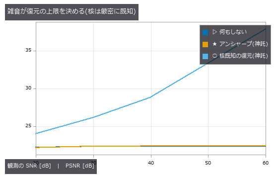
↑ How Much Camera Shake Can Be Undone — Make the Kernel, Apply It, Invert It, Compare ―― A known linear blur kernel applied and inverted, with the ceiling set by noise and by kernel estimation error. Without noise the image recovers from 22.38 to 56.41 dB; at 20 dB SNR the gain is 1.82 dB. A kernel angle off by 19.4 degrees is beaten by doing nothing, and undoing rotational blur with a single kernel makes the centre of rotation worse by -49.41 dB.

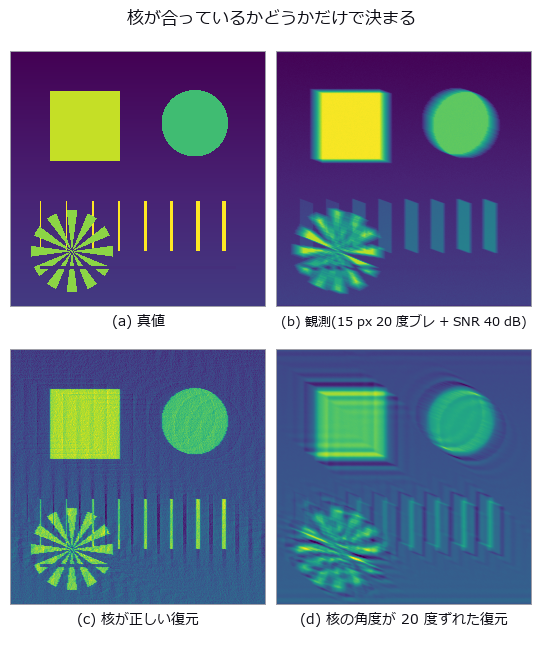
↑ The measurement ―― 4 枚目は「復元した」形をしているが、ゼロ点(観測そのもの)より悪い。絵の見た目では区別できない。 (figure labels are in Japanese; the numbers are the same)

↑ 交点が現場で効く数字。

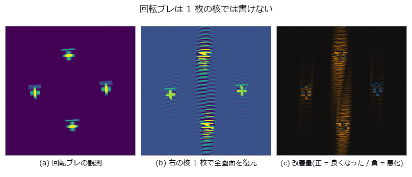
↑ 核を作った右側だけが正。

py -3.11 examples/poc_camera_shake_deblur.py

Source: examples/poc_camera_shake_deblur.py

This run produced 4 figures in total - see them all

Ops used (notes): psnr · reflect · ssim · unsharp · vol_richardson_lucy

No.2026.062 —— Pseudo-colour changes what the reader decides — counting edges that are not there

↑ Pseudo-colour changes what the reader decides — counting edges that are not there ―― A smooth field with provably zero steps was painted and the false edges counted in CIE L and CIEDE2000: jet raises 3, hsv 4, while viridis and gray raise none. Their positions follow in closed form from the sRGB transfer function and the CIE Y weights — jet's lightness reversals are predicted at 0.3750 / 0.4490 / 0.6250 and measured at 0.3750 / 0.4492 / 0.6250 (max error 0.0002). A real step only out-shouts the false edges above 0.296 %FS with jet versus 0.050 %FS with viridis, matching a prediction made from the colormap LUT alone: jet demands a 5.9x taller step. The value-to-colour mapping matters more than the palette — over a 4.3-decade 1/r^2 field the effective number of distinguishable levels goes from 1.4 (linear) to 76.0 (rank) — and a single outlier costs log 41 % of them (27.4 to 16.3) while percentile and rank are untouched.*

↑ The measurement ―― 平らなら偽の境目は立たない。jet と hsv の山がそのまま『見えてしまう帯』になる。 (figure labels are in Japanese; the numbers are the same)

↑ この回の図

↑ jet の輪が偽の境目。

↑ 左は範囲外と『ちょうど端』が同じ色。

↑ 番号の大小に意味は無いのに、連続マップは『近い番号 = 近い領域』と読ませる。

py -3.11 examples/poc_colormap_readability.py

Source: examples/poc_colormap_readability.py

This run produced 14 figures in total - see them all

Ops used (notes): delta_e_map · percentile · rgb_to_lab

No.2026.118 —— The Fly's Compound Eye Is a Light-Field Sensor — Neural Superposition Pays Only Up to the Knee

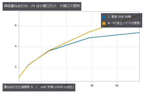
↑ The Fly's Compound Eye Is a Light-Field Sensor — Neural Superposition Pays Only Up to the Knee ―― A 9×9 plenoptic synthesis of the ommatidial array, measuring the SNR gain when the same point is pooled over N ommatidia. For small apertures √N holds almost exactly (N=5: 2.25 vs 2.24), but for large ones the interpolation error does not average out and the gain saturates (N=49: 5.33 vs 7.00). The fly's six-fold pooling of R1–R6 sits below the knee. Depth comes from the array (near +1.998, far +0.499 against true 2.00 / 0.50), and a minority occluder is seen through by median pooling (RMS on hidden pixels: single view 0.237 → mean 0.065 → median 0.025).

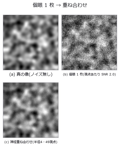
↑ The measurement (figure labels are in Japanese; the numbers are the same)

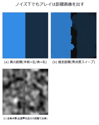
↑ この回の図

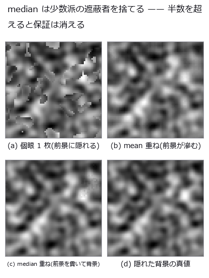
↑ この回の図

py -3.11 examples/poc_compound_eye.py

Source: examples/poc_compound_eye.py

This run produced 4 figures in total - see them all

Ops used (notes): lf_all_in_focus · lf_aperture_mask · lf_depth_from_focus · lf_plenoptic_design · lf_subaperture · lf_synthesize · lf_synthetic_aperture · median

No.2026.010 —— Where CT Reconstruction Starts to Break as Projections Are Removed

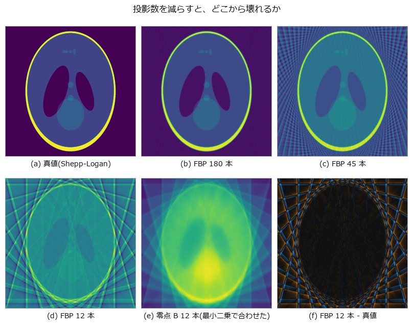
↑ Where CT Reconstruction Starts to Break as Projections Are Removed ―― Shepp-Logan re-imaged with 180 down to 12 projections, FBP placed beside two nulls: a blank image and unfiltered back-projection. With 12 projections FBP (RMSE 0.2576) is worse than the blank image (0.2420). A check that never looks at the reconstruction — the row sums of the sinogram — caught a -3.34 % mass loss that RMSE could not see; fixing the ramp filter's DC bin brought it to -0.0099 %.

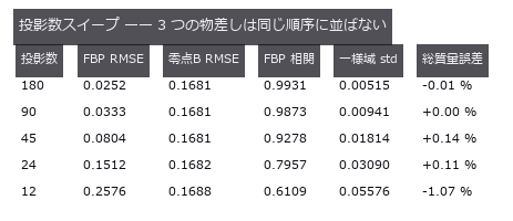
↑ The measurement ―― RMSE で見ると 12 本は空白画像 0.2420 より悪い。相関とストリークは別のことを言う。 (figure labels are in Japanese; the numbers are the same)

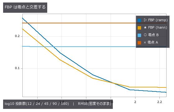
↑ 零点 A = 空白画像、零点 B = 無フィルタ逆投影(どちらも水平・ほぼ水平)。

py -3.11 examples/poc_ct_fidelity.py

Source: examples/poc_ct_fidelity.py

This run produced 3 figures in total - see them all

Ops used (notes): backproject_sinogram · ellipse_phantom · ellipse_sinogram · filtered_backprojection · projection_angles · radon_transform · rmse · ssim · stat_correlation

No.2026.011 —— Removing Haze — Ground Truth From the Scattering Model, Transmission and Airlight Scored Apart

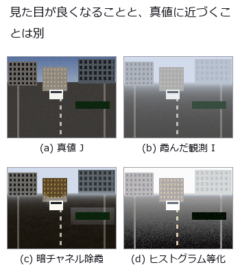
↑ Removing Haze — Ground Truth From the Scattering Model, Transmission and Airlight Scored Apart ―― A hazy image built from depth, airlight and extinction so that the true transmission and the true scene are both known, then dehazed and scored. The overall +4.04 dB hides a -1.49 dB degradation of the near field covered by +4.03 dB mid and +11.28 dB far. Above 782 m visibility dehazing does harm, and adding noise raises PSNR (an accidental cancellation).

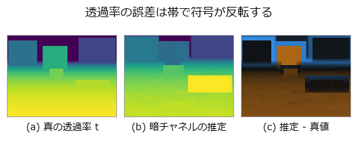
↑ The measurement ―― 空では過大評価(明るい側)、近景では過小評価(暗い側)。全体の平均バイアスでは打ち消し合って見えない。 (figure labels are in Japanese; the numbers are the same)

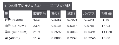
↑ 全体 +4.04 dB の正体。

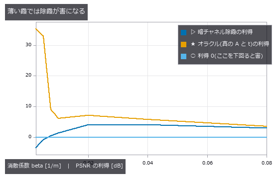
↑ 左端(薄い霞 = 視程が長い側)で利得が 0 を割る。

py -3.11 examples/poc_dehazing.py

Source: examples/poc_dehazing.py

This run produced 4 figures in total - see them all

Ops used (notes): clahe · equalize · image_entropy · joint_bilateral · psnr · rank_image · ssim

No.2026.016 —— Ranging by Counting Photons — How Many for How Many Millimetres?

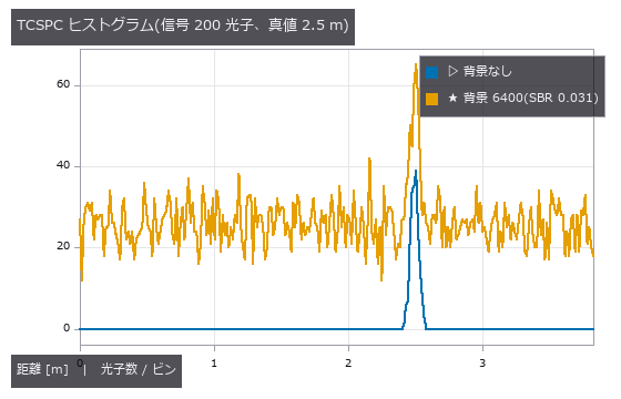
↑ Ranging by Counting Photons — How Many for How Many Millimetres? ―― Range read from an arrival-time histogram built by bin-integrating a Gaussian at the round-trip time and drawing Poisson samples. With 200 photons the raw peak position errs by 11.02 mm and the gated centroid by 2.29 mm, riding the 31.83 mm/√N bound at 1.00 to 1.07x. With background the plain centroid collapses by two orders (564 mm at SBR 0.031), and the family's recommended Gaussian fit at 8.82 mm loses to a gated centroid a user can write in six lines.

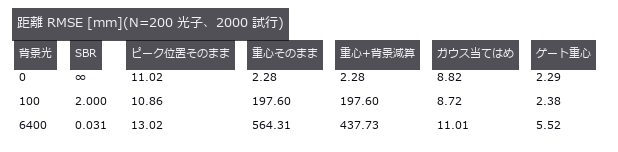
↑ The measurement ―― 背景が無ければ素の重心で足りる。背景が入ると 2 桁崩れ、docstring が勧める背景減算でも戻らない。 (figure labels are in Japanese; the numbers are the same)

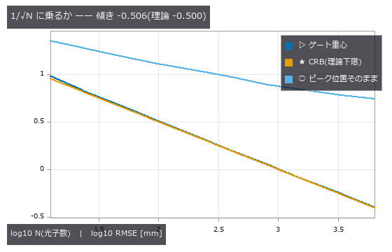
↑ ゲート重心は CRB に寄り添って落ちる。

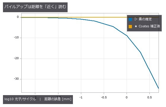
↑ 素の推定は μ にほぼ比例して手前へずれる(5 光子/サイクルで -34.5 mm)。

py -3.11 examples/poc_dtof_ranging.py

Source: examples/poc_dtof_ranging.py

This run produced 4 figures in total - see them all

Ops used (notes): dtof_cube_depth · dtof_cube_simulate · dtof_depth · gaussian · median · tcspc_background_subtract · tcspc_coates_correct · tcspc_simulate

No.2026.119 —— The Fly's Visual Front End as a Chain of Operators — Turning and Walking Through a Synthetic Sky, What Can and Cannot Be Read

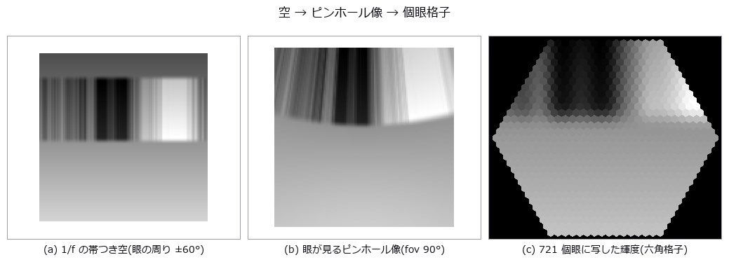
↑ The Fly's Visual Front End as a Chain of Operators — Turning and Walking Through a Synthetic Sky, What Can and Cannot Be Read ―― One eye assembled from a 721-ommatidium hexagonal lattice → acceptance function → lamina DC removal → Hassenstein-Reichardt correlators → HS opponent sum, turning under a 1/f banded sky. The direction and waveform of self-rotation are readable (correlation with the true yaw rate +0.785, +0.880 with a membrane low-pass, sign agreement 0.92), but skipping the lamina DC removal makes the correlator emit a DC × high-pass ripple and the correlation drops to +0.504. Walking forward without turning, the full-field readout turns into a −0.689 'rotation'; restricting to the upper field still leaks −0.221 because acceptance functions straddle the horizon (0.000 above el = 2Δρ). The opponent ratio discards speed, so a 1.4°/s flow from a dome 20 m away reads −0.612. The LGMD η peak comes α·l/|v| before collision (−0.1570 s, predicted −0.1567 s) at θ = 23.97° (predicted 24.02°; 24.6° for the exact subtense of a sphere, a quartic root), the sphere τ rides d/|v| with RMS 1e-5 s, and the disk formula misapplied to a sphere reads cos²(θ/2) = 0.75× at 60°. Twelve grating directions give DSI 0.798 with preferred direction 0°.

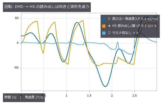
↑ The measurement ―― 相関 +0.785(膜 LP つき +0.880、ラミナ段なし +0.504)。対向比は符号の一致度なので、尺度 k は最小二乗で合わせてある。 (figure labels are in Japanese; the numbers are the same)

↑ 偏り: 全視野 -0.689 / 上半 el>0 -0.221 / el>2Δρ +0.000 / ドーム -0.612

↑ ピーク -0.157 s(予測 -0.157 s)、θ_peak 24.0°(予測 24.0°)。

↑ 球式は RMS 0.00001 s で真値に乗る。

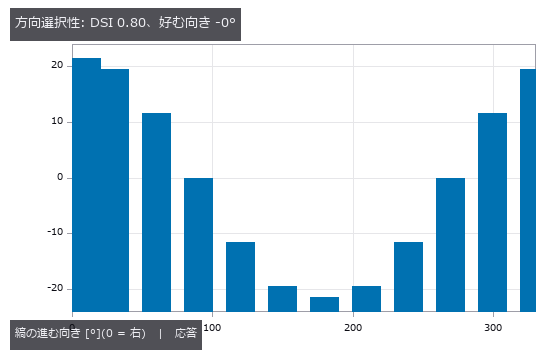
↑ 負の応答(逆向き)は fly_dsi が 0 に切る。

py -3.11 examples/poc_fly_vision.py

Source: examples/poc_fly_vision.py

This run produced 6 figures in total - see them all

Ops used (notes): fly_dsi · fly_emd_response · fly_hex_lattice · fly_hex_resample · fly_hs_readout · fly_lgmd_eta · fly_sky_1f · fly_tau_from_expansion

No.2026.019 —— Focus Stacking — The All-in-Focus Image and the Depth Map Are Different Things

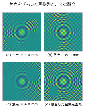
↑ Focus Stacking — The All-in-Focus Image and the Depth Map Are Different Things ―― An all-in-focus image and a depth map pulled from 15 frames blurred by the closed-form circle of confusion. The all-in-focus image reaches 35.89 dB (null 20.98 dB), yet the depth from the same fusion loses to the null by 8x (0.13x) in textureless regions. A relative confidence scores 0.9923 there, higher than the 0.9630 of textured regions; rejecting by absolute value (23600x apart) brings the RMS from 1.505 to 0.878 mm.

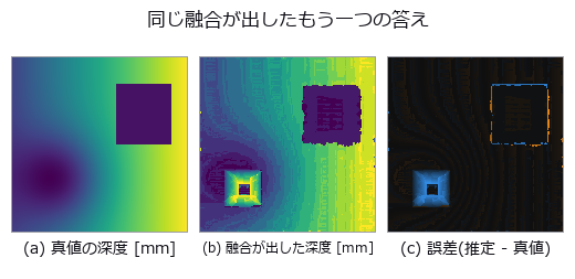
↑ The measurement ―― 左下の無テクスチャの四角だけ、誤差が掃引全域にばらけた乱数になっている(段差帯のハローも見える)。 (figure labels are in Japanese; the numbers are the same)

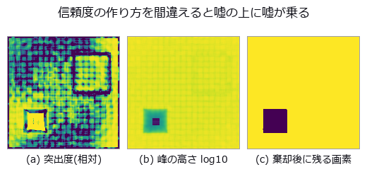
↑ 左下の無テクスチャの四角が、相対量(0.90-1.00 に切って表示)では最も明るい = 自信ありに見え、絶対量(対数)でだけ「何も見えていない」と出る。

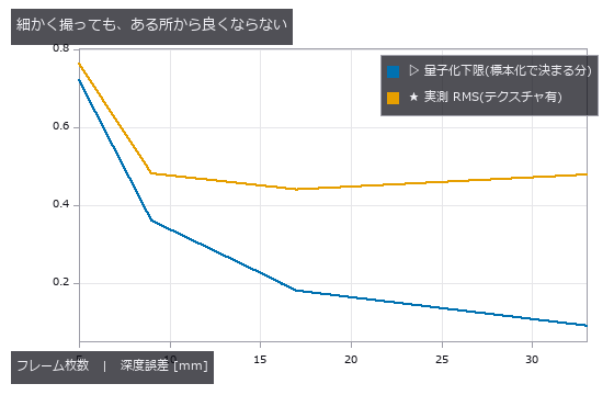
↑ 2 本が離れていく = 残りの誤差は標本化ではなく焦点評価が持っている。

py -3.11 examples/poc_focus_stacking.py

Source: examples/poc_focus_stacking.py

This run produced 4 figures in total - see them all

Ops used (notes): csi_height_map · defocus_blur · dilation_circle · fuse · gauss_filter · laplace · mean_image · optical_camera · psnr · sobel_amp · xcv2_lap_var

No.2026.023 —— Depth From a Light Field — A Light Field of Known Depth, Confronted With Its Nulls

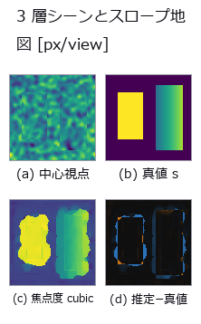
↑ Depth From a Light Field — A Light Field of Known Depth, Confronted With Its Nulls ―― A 9×9 light field rendered by analytic inverse mapping, with focus-measure, EPI-slope and two-view block matching scored against the true slope map. The winner beats the constant null by 22x, but beats two-view matching — which uses only 2 of the 81 views — by just 1.6x, and only with cubic interpolation. The default linear interpolation snaps to integer slopes, reading a true 1.30 as 1.4750 (11.9 % in depth).

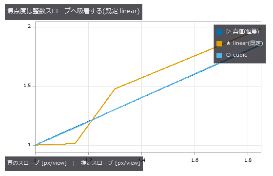
↑ The measurement ―― linear は 1.08/1.15 を 1.0 へ、1.85 を 2.0 側へ引く。cubic は恒等線に乗る。生成側の補間はゼロ(Fourier シフト)。 (figure labels are in Japanese; the numbers are the same)

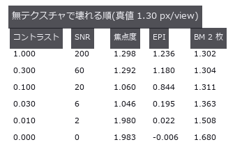
↑ EPI は SNR 20 で既に -35 %。

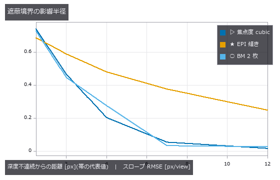
↑ 境界から 5 px 離れれば内側の水準に戻る。

py -3.11 examples/poc_lightfield_depth.py

Source: examples/poc_lightfield_depth.py

This run produced 4 figures in total - see them all

Ops used (notes): lf_depth_from_focus · lf_disparity_to_depth · lf_epi · lf_epi_slope · lf_refocus

No.2026.105 —— Deblurring a Real Photograph — Three Rulers, Three Different Winners

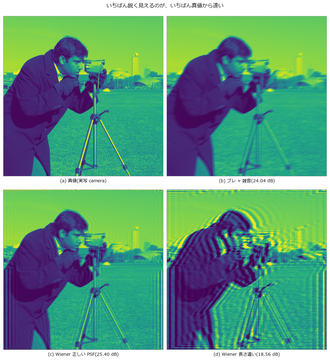
↑ Deblurring a Real Photograph — Three Rulers, Three Different Winners ―― The truth here is a real photograph (scikit-image camera, CC0) and only the degradation is planted: a straight 11-pixel blur at 20 degrees plus noise of sigma 0.004. Doing nothing scores 24.04 dB, and a Wiener filter at the commonly used nsr of 0.005 scores 23.66 — it loses to the null. Stopping there would be misrepresenting the method: sweeping nsr gives 19.18 dB at 0.0005 and 25.40 dB at 0.02, so a fixed knob is not a comparison at all. The knob moves the result by 6.22 dB while deconvolving at all is worth 1.36 dB, a factor of 4.6 — the setting matters more than the method. Applying three rulers to the same seven results puts three different methods first: PSNR picks the correct-PSF Wiener at 25.40 dB, gradient energy picks motion_deblur at 0.2986, which is 1.54 times the truth's own 0.1936 — an image sharper than the truth wins — and blur_effect picks unsharp. The methods those reference-free rulers choose cost 4.98 dB and 3.26 dB against the best. In fairness, blur_effect does rank the truth itself above every method: it measures blur correctly and still loses you three decibels when used to choose. Mistaking the blur length as 21 instead of 11 costs 5.48 dB against doing nothing while raising the gradient energy to 1.37 times the truth, so it looks like it worked. The cliffs: at sigma 0.016 the gain falls to 0.05 dB, and the gain over blur length peaks at 5 pixels, falling at both ends because a short blur has little to remove and a long one has destroyed the information.

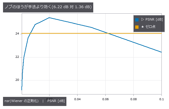
↑ The measurement ―― 固定した nsr で比べると、正しい PSF でもゼロ点に負ける。 (figure labels are in Japanese; the numbers are the same)

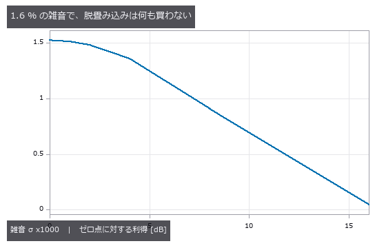
↑ σ=0 で +1.52 dB、σ=0.016 で +0.05 dB。

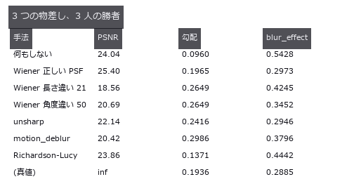
↑ 参照なし指標が選ぶ手法は PSNR で 3〜5 dB 劣る。

py -3.11 examples/poc_real_deblur_honesty.py

Source: examples/poc_real_deblur_honesty.py

This run produced 4 figures in total - see them all

Ops used (notes): iv_motion_deblur · iv_richardson_lucy · iv_unsharp_deblur · psnr · reflect · sk_blur_effect · unsharp

No.2026.039 —— Does Super-Resolution Add Information? Downsample With the Truth in Hand, Restore, Count

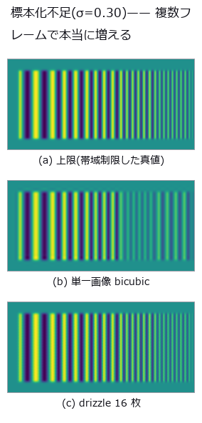
↑ Does Super-Resolution Add Information? Downsample With the Truth in Hand, Restore, Count ―― Observations made by downsampling the truth, with single-image upscaling, iterative back-projection and drizzle scored on a resolution table. No single-image upscaler beats the bicubic null by more than +0.036 dB. Drizzling 16 sub-pixel-shifted frames gains +13.96 dB in the undersampled condition, and the modulation of a period-6 pattern beyond Nyquist rises from 0.03 to 0.38.

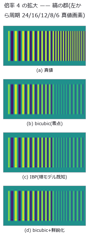
↑ The measurement ―― 鮮鋭化だけがナイキスト(周期 8)より細かい列にも縞を作る。それは分解能ではなく無い縞。 (figure labels are in Japanese; the numbers are the same)

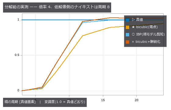
↑ IBP は周期 12 以上の落ちた変調を戻すが、8 より細かい列は1 本も戻らない(順モデルの零空間)。

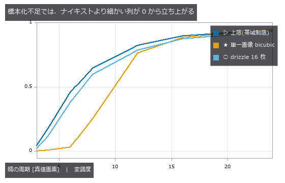
↑ 上限の線がレンズの許す限界。

py -3.11 examples/poc_superresolution_limits.py

Source: examples/poc_superresolution_limits.py

This run produced 4 figures in total - see them all

Ops used (notes): drizzle_resample · piv_cross_correlate · psnr · ssim · unsharp · vol_fft_lowpass · vol_resize · volume_downsample

No.2026.135 —— Holding a Course with a Fly's Optic Lobe Alone — From the Lamina to the Steering, Without Learning

↑ Holding a Course with a Fly's Optic Lobe Alone — From the Lamina to the Steering, Without Learning ―― A vehicle whose heading drifts under a disturbance, carrying nothing but a compound eye and closed-form circuitry, holds its course: the fly's optomotor response built out of fullseye operators alone and measured next to a ground-truth gyro. Every stage is a closed form and nothing is trained: hexagonal sampling (fly_hex_resample), lamina adaptation and band-pass (fly_lamina_filter), the ON/OFF split (fly_onoff_split), direction selectivity in all six lattice directions (fly_t4t5_field), the local flow (fly_flow_from_directions), a linear fit against the matched filter (fly_matched_filter / fly_egomotion_from_flow), and a six-neuron, eight-synapse steering circuit run as conductances (graph_conductance_states). Each stage has an exact identity: brightening the whole scene ten thousand times leaves the lamina output unchanged (Weber, 7e-16), the three-arm T4 model with Haag et al. 2016's verbatim constants (tau = 250 ms, k = 5/5/10) returns the paper's 24.9636 and 0.8195 on its two-column stimulus, and the paper's claim that the two mechanisms are complementary becomes a product identity (4.161 x 7.321 = 30.461 = the whole model) that holds to machine precision; the matched filter's 1.7 rad/s comes back to nine digits. The limits are measured too: on the classical striped drum the estimate tracks a time-varying rotation at 0.976 correlation, in a natural 1/f scene at 0.897, and the single calibration gain it needs is 2.64 on the drum against 6.76 and 7.88 in natural scenes - 3.0x between kinds of scene and 1.16x between two scenes of identical statistics, because a correlation detector reports contrast-weighted motion rather than velocity. A single 80-degree eye measuring the same +0.5 rad/s across twelve scenes scatters by 1.05 of its mean and gets the sign of the rotation wrong in four of them; merging three eyes into 250 degrees with fly_eye_merge drops the scatter to 0.44 and the sign errors to zero - the width of a compound eye is not decoration. In closed loop (calibrated in scene A, flown in an unseen scene B) the open loop drifts 51 degrees, the visual reflex 33, and the ground-truth gyro 23: a reflex has no absolute heading and cannot null the drift, which is where the central complex would come in. Writing the steering on the connectome side gives the same 33 degrees, and the membrane potential is a convex combination of the reversal potentials so it cannot diverge. No data ships; the scenes are generated from seeds by fly_sky_1f.

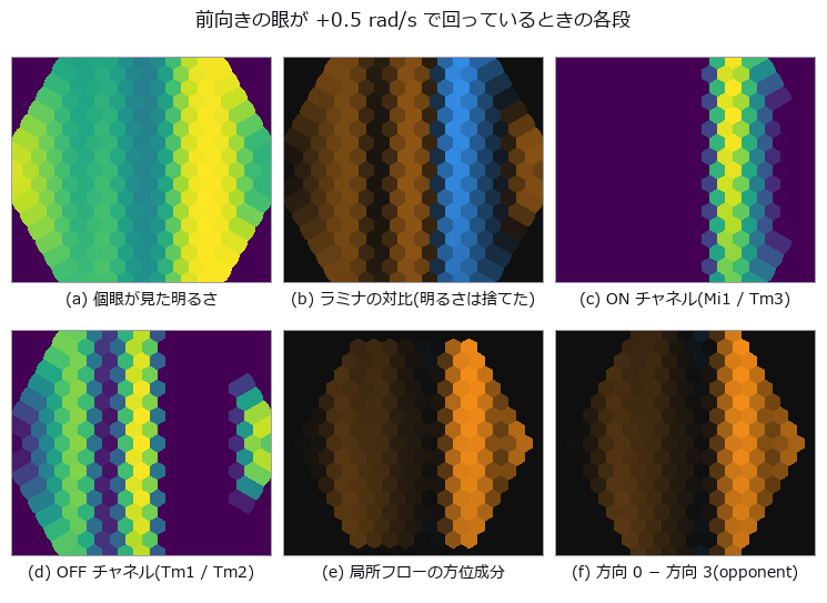
↑ The measurement ―― left to right, top to bottom: what the ommatidia see, the lamina's contrast (brightness thrown away), the ON and OFF channels, and the direction-selective field read as a local flow. The eye is turning at 0.5 rad/s in a 1/f panorama; nothing here was trained. (figure labels are in Japanese; the numbers are the same)

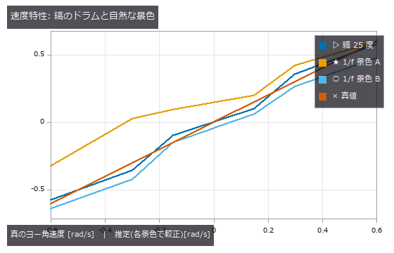
↑ each scene is fitted with its own single gain; the striped drum is nearly linear, and a natural 1/f scene needs a gain 3.0x larger — a correlation det…

↑ a narrow eye is at the mercy of whichever few large features are in front of it: over eight scenes of identical statistics it scatters and gets the si…

↑ the disturbance has a steady bias, so the open loop drifts away; the optomotor reflex cuts the drift but cannot null it — a reflex has no absolute hea…

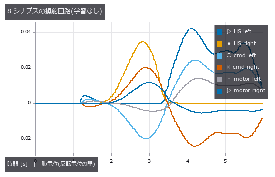
↑ the wiring is written by hand as a synapse table and run as a conductance circuit; the state is a convex combination of the reversal potentials, so it…

py -3.11 examples/poc_fly_optomotor_steering.py

Source: examples/poc_fly_optomotor_steering.py

This run produced 7 figures in total - see them all

Ops used (notes): fly_egomotion_from_flow · fly_eye_merge · fly_flow_from_directions · fly_hex_lattice · fly_hex_resample · fly_lamina_filter · fly_matched_filter · fly_onoff_split · fly_sky_1f · fly_t4t5_field · graph_conductance_states · graph_from_synapses

No.2026.148 —— The Exact Distance at Which Detail Vanishes, and the Area of a Changing Shape

↑ The Exact Distance at Which Detail Vanishes, and the Area of a Changing Shape ―― Both a picture that mixes high and low frequencies and a shape that morphs smoothly carry exact truths that can be measured straight off the image - and the customary way of making them is the one that misses those truths. The first concerns orthogonality. Splitting an image into low and high parts with an ideal frequency mask makes the two exactly orthogonal, so the energies add: across four cut-off frequencies the relative discrepancy in E(low) + E(high) - E(original) is 1.9e-16. The textbook construction - blur with a Gaussian, call the remainder the high part - misses by 0.53 % to 3.10 %, even though both reconstruct the original exactly when added back: being invertible and being orthogonal are different properties. The discrepancy is also not monotone in the blur: the worst case is the weakest blur and the best is in the middle of the range, so neither strengthening nor weakening it fixes the problem. The second concerns distance. Binning k pixels - what moving away does - has the transfer function sin(pi f k)/(k sin(pi f)), which is exactly zero when f times k is an integer, so a pattern of period p pixels vanishes exactly when binned at p pixels (1.4e-14 over five periods). More strongly, the binned picture can be written pixel by pixel in closed form - the amplitude and the fact that the binned pixel's centre shifts by (k-1)/2 - agreeing to 2.8e-14 over every pixel for bin widths 1 through 48. The third concerns shape. Interpolating polygon vertices linearly makes the enclosed area an exact quadratic in t, so three frames predict all of them (2.4e-15 across three shapes), and this survives measurement from the picture: rasterising the polygon and counting brings the deviation from 1.10 % on a 128 grid down to 0.053 % on a 512 grid with each pixel split four ways - and splitting a pixel into 4x4 gives exactly the same number as using a four times finer grid. The fourth is where measurement from a picture breaks. Morphing to the same polygon with its vertices reversed makes the signed area linear in t, vanishing at t = 0.5 where the polygon collapses to a line, and the quadratic prediction holds to 3.4e-15; but a picture only yields positive area, so the parabola folds and the three-frame prediction is off by exactly one quarter of the maximum - measured at 25.0 % for two different shapes. Even the size of the error has a closed form. The fifth pairs two exact spline properties: Catmull-Rom passes through its control points at distance 0.0e+00, while a Bezier curve does not pass through them but never leaves their convex hull (401 of 401 points across four sets) - exactly complementary guarantees. Three predictions were wrong and have been left in: that the bin width at which a hybrid image switches could be predicted from the cut-off frequency as 1/(2 fc), when in fact tripling the cut-off barely moves the measured switch because what governs it is the period the high-frequency picture actually contains; that the Gaussian discrepancy would grow with the blur; and that reading amplitude off the picture's maximum and minimum would match the closed form, when at a bin width of six it reads 20.7 % low because the pixels never land on the crest - the formula is right even where no pixel sits. No new operator was added.

↑ The measurement ―― 低い周波数に粗い模様、高い周波数に細かい模様を入れた 1 枚を、束ねながら見たもの。束ねるのは「遠ざかる」ことで、細かいほうが先に消える。ただし ★いつ消えるかは遮断周波数では決まらない —— 下の数表の「外した予言」を参照。 (figure labels are in Japanese; the numbers are the same)

↑ どちらも足せば元に戻る(再構成の誤差は両方 1e-13 未満)。

↑ k = 24 と k = 48(f·k が整数)で 厳密に 0、その間では戻る。

↑ 閉形式なら 2.4e-15。

↑ 薄い折れ線が制御点をつないだもの、濃い線が Catmull-Rom。

↑ The animation ―― 6 角形が別の 6 角形へ変わって戻るところ。★見た目は連続に変わるが、囲む面積は t の 厳密な 2 次式に乗っている(次の図)。

py -3.11 examples/poc_vanishing_detail_and_morphing_area.py

Source: examples/poc_vanishing_detail_and_morphing_area.py

This run produced 14 figures in total - see them all

Ops used (notes): convex_hull · gauss_filter · morph

The Time-as-3-D Wing — A Video Is One Volume

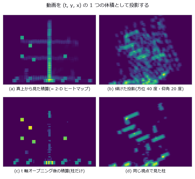
Treat a 2-D video as one (t, y, x) volume and the 3-D ops — connected components, isosurfaces, region properties — work along time unchanged. Merging colonies become a Y in space-time, passing vehicles become bands in a (t, x) image, a wavefront's arrival time becomes an isosurface. The 14 exhibits here demonstrate exactly that.

The time axis also brings its own traps. Rounding onto the frame grid always delays; pixel area makes merging look early. Mislinks come in two opposite kinds, so a single error rate cannot say which way the diffusion coefficient is wrong. Template tracking drifts quietly before it ever loses the target, and all 152 drifted frames report 'found'.

The motion-magnification exhibit carries the most candid conclusion in the room: exact to machine precision up to a magnification of 200, and of no help for measurement. Magnification is a tool for showing people, not for measuring.

No.2026.055 —— Modal identification from video — frequency survives to the end, damping lies first

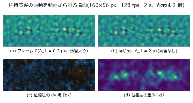
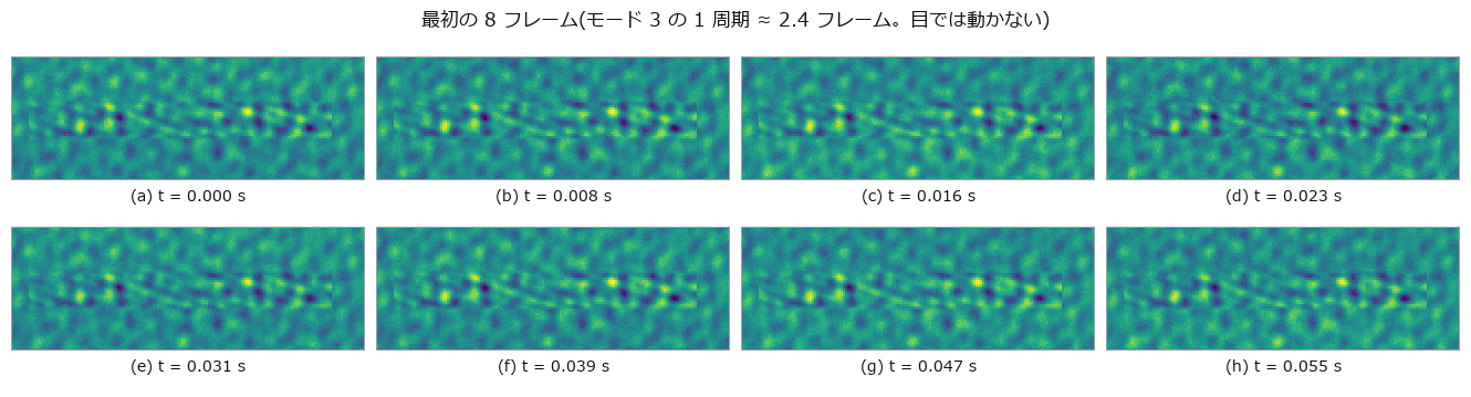
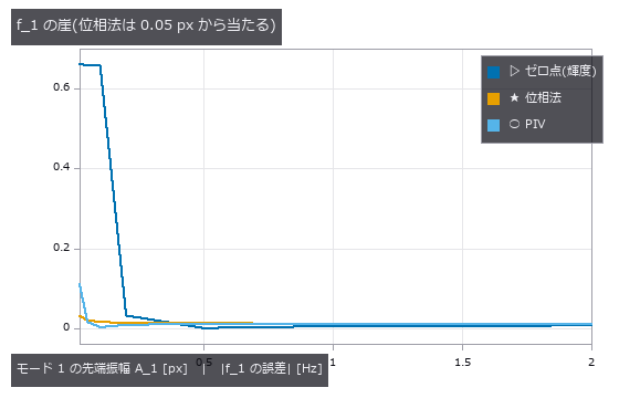
↑ Modal identification from video — frequency survives to the end, damping lies first ―― A cantilever beam (closed-form Euler–Bernoulli modes) decaying freely in three modes is rendered into video with sensor noise, 100 Hz lighting flicker, camera shake and rolling shutter, then identified with phase-based displacement (phase_displacement) and PIV (piv_cross_correlate). All three natural frequencies come out within 0.06 Hz, but the damping ratio of mode 1 from the very same series is 0.0778 (half-power), 0.0188 (envelope) or 0.0181 (fit) against a true 0.02. Sweeping the amplitude from 0.02 to 2 px, the quantities break in the order f → ζ → MAC_2 → MAC_3: at 0.02 px the phase method still has f_1 within +0.030 Hz while ζ_1 is 0.23 of the truth. At 48.5 fps the flicker alias lands exactly on f_1 = 3.00 Hz; a single-pixel brightness zero-point cannot report ζ at all, while the phase method survives at 0.0191.

↑ The measurement (figure labels are in Japanese; the numbers are the same)

↑ この回の図

↑ この回の図

↑ この回の図

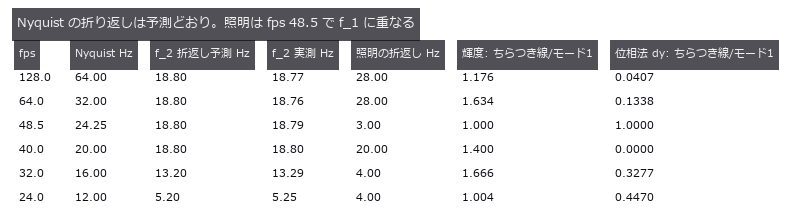
↑ この回の図

py -3.11 examples/poc_beam_modal_video.py

Source: examples/poc_beam_modal_video.py

This run produced 13 figures in total - see them all

Ops used (notes): envelope · phase_displacement · piv_cross_correlate · temporal_bandpass

No.2026.060 —— The Cold-Chain Temperature Record — Where You Taped the Logger Is the Verdict

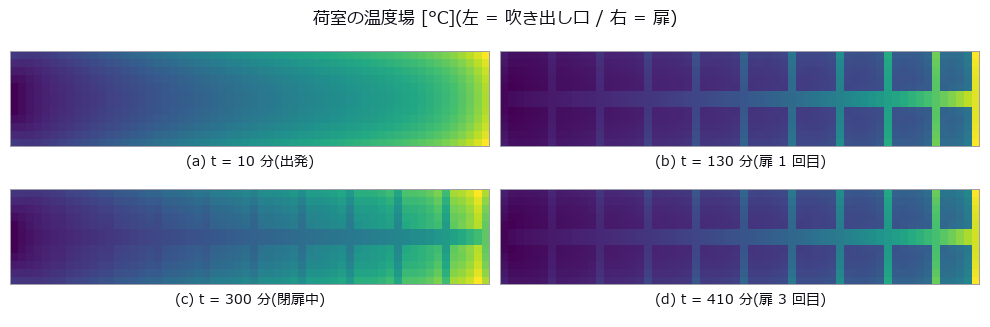
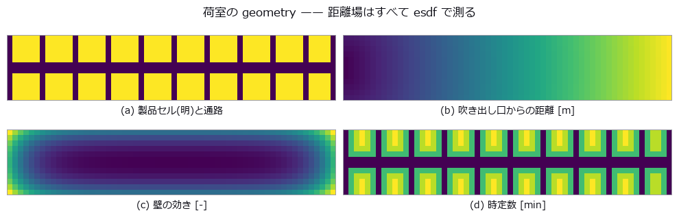
↑ The Cold-Chain Temperature Record — Where You Taped the Logger Is the Verdict ―― Twelve hours of a 12.0 m x 2.4 m reefer hold, built as a single (t, y, x) volume of 720 min x 60 x 12 cells with known closed-form physics: distance from the supply vent, infiltration from each of the four walls, five door-opening pulses, and first-order thermal lag (5 min for air, 64-91 min for product). 108 of 490 product cells (22.0 %) truly fail, yet a single logger taped in the product reports PASS for 82.4 % of the placements. Turning the causes off one at a time separates the failure modes: walls alone give 95.5 % false passes and 0.0 % false alarms, while walls off and doors on drop true failures to 2.0 % but raise false alarms to 3.5 % — and a logger in the product then passes 100 % of the time, because short pulses never enter the product. The cliffs can be predicted on paper: the time-constant cliff measured at 19-138 min matches a two-stage (hold air + logger) model within 18 % relative, and the sampling-interval and 0.5 K quantisation cliffs match their predictions exactly. Converted to "minutes allowed at 12 °C", the three metrics computed from the same record differ by 4.6x (60 / 276 / 197 min) and disagree on the verdict at 82 of 720 placements (11.4 %).

↑ The measurement (figure labels are in Japanese; the numbers are the same)

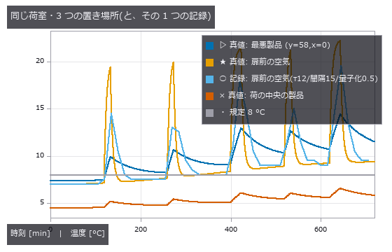
↑ 扉前の空気は跳ねるが製品には届かない。

↑ この回の図

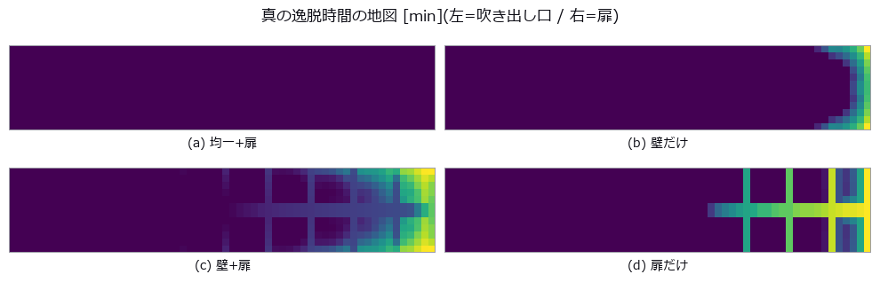
↑ この回の図

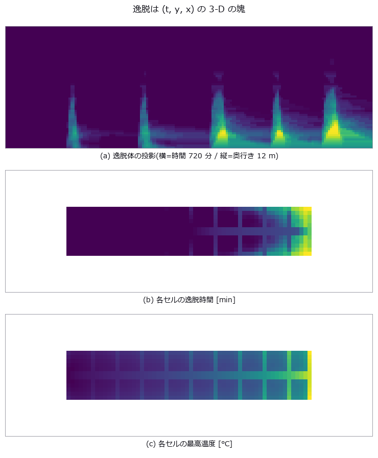
↑ 1 枚目は render_volume_projection を幅方向から掛けた xray 投影(明るいほど幅方向に厚い)。

py -3.11 examples/poc_cold_chain_excursion.py

Source: examples/poc_cold_chain_excursion.py

This run produced 16 figures in total - see them all

Ops used (notes): esdf · integrate_funct_1d · quantize · render_volume_projection · sample_funct_1d · vol_label · vol_label_shape_stats · vol_mip · vol_profile_line · vol_region_props

No.2026.095 —— Measuring the Growth, Not the Width — Rephotographing the Same Wall Changes What the Error Is

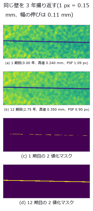
↑ Measuring the Growth, Not the Width — Rephotographing the Same Wall Changes What the Error Is ―― A wall at 1 px = 0.15 mm, rephotographed for twelve epochs over three years, with a crack opening at a true 0.040 mm/yr. Thresholding and counting pixels understates the width by 25.0 % yet overstates the growth rate by +153.0 %, and invents +0.0117 mm/yr of growth in a control where the width is frozen (the culprit is blur, isolated by switching one nuisance at a time). Integrating the intensity deficit gives +3.1 % on the rate and +0.0005 mm/yr on the control. The thresholded rate swings from 0.0241 to 0.1038 mm/yr on initial width alone — it depends on whether a one-pixel step happens to fall inside the observation window.

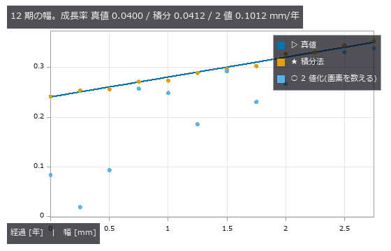
↑ The measurement ―― 2 値化は幅の偏りより期ごとの跳ねが問題。跳ねの正体はぼけと画素位相で、4 節と 3 節で分けて数える。 (figure labels are in Japanese; the numbers are the same)

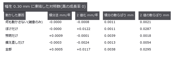
↑ ここに出る傾きはすべて『見かけの成長』。

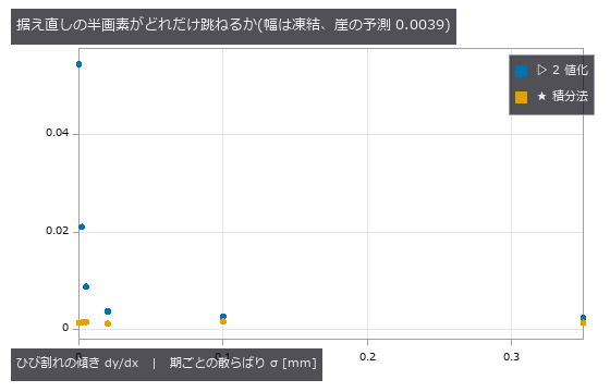
↑ 傾きが 0 に近いほど列方向の画素位相が揃い、2 値化は画面ごと 1 画素単位で跳ぶ。

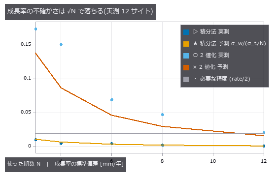
↑ 横線を下回った時点で 0.040 mm/年 を 2σ で言える。

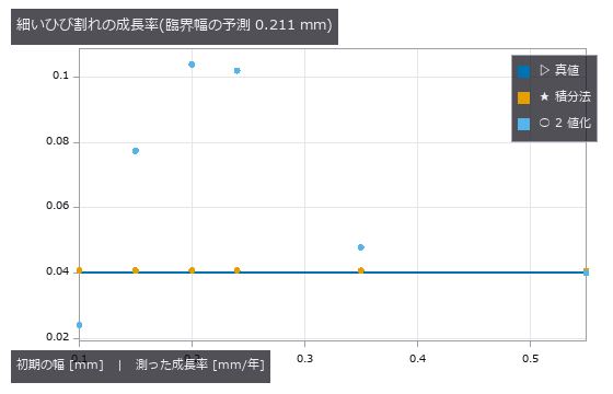
↑ 2 値化は臨界幅より細いと 0(未検出)。

py -3.11 examples/poc_crack_width_timeseries.py

Source: examples/poc_crack_width_timeseries.py

This run produced 10 figures in total - see them all

No.2026.026 —— Micro-Vibration of a Structure From Video — Does Motion Magnification Help You Measure?

↑ Micro-Vibration of a Structure From Video — Does Motion Magnification Help You Measure? ―― A vibration of known amplitude 0.02 px at 3.7 Hz, synthesised to test whether motion magnification helps measurement. Exact to machine precision up to α = 200. But magnification does not improve measurement precision — multiplying the phase by α multiplies the noise by α. On a cantilever, phase correlation returns 0.15 px, the area average of 0.30 and 0.00 px, a number that exists nowhere.

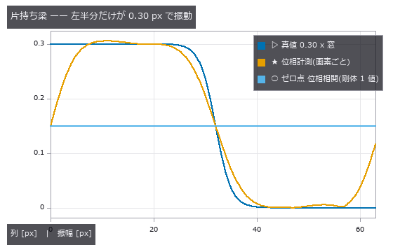
↑ The measurement ―― 剛体を仮定する位相相関が返す 0.150 px は 0.30 と 0.00 の面積平均で、どの列の真値とも違う。 (figure labels are in Japanese; the numbers are the same)

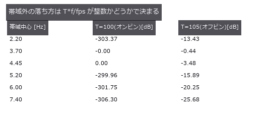
↑ 3.7 Hz を含む帯だけが 0 dB。

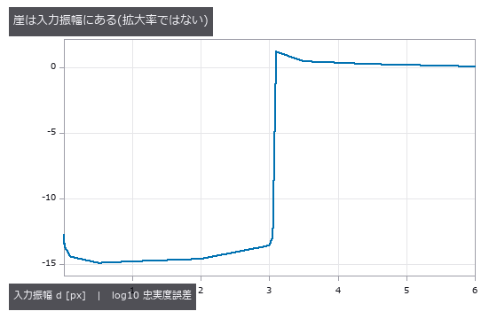
↑ 3.05 px までは機械精度、3.10 px で崩壊。

py -3.11 examples/poc_motion_magnification.py

Source: examples/poc_motion_magnification.py

This run produced 4 figures in total - see them all

Ops used (notes): band_snr · displacement_series · motion_magnify · phase_displacement · synthesize_translation · temporal_band_power · temporal_bandpass

No.2026.030 —— Particle Tracking as a (row, column, time) Volume — Mislinks Come in Two Directions

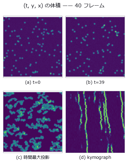
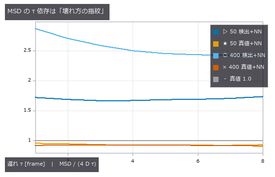
↑ Particle Tracking as a (row, column, time) Volume — Mislinks Come in Two Directions ―― A video of 400 particles tracked, with the diffusion coefficient D read from the trajectories. Ambiguous mislinks pull D down to 0.925x; mislinks caused by missing targets push it up to 3.429x in the same video — one error rate cannot tell you the direction. What helps is not a one-to-one constraint but a single line imposing a maximum link distance (3.429 → 1.304).

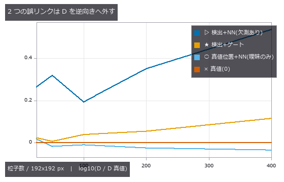
↑ The measurement ―― 縦軸は常用対数(0 が真値)。欠測は遠い他人を掴んで D を上げ、曖昧は近い相手を選んで D を下げる。上限距離のゲート 1 行で上向きの暴走が 1/2.6 に。 (figure labels are in Japanese; the numbers are the same)

↑ 真値で割った比。

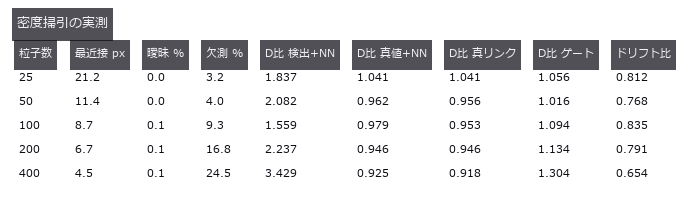
↑ 曖昧と欠測を分けて数えると、D の外れる向きが説明できる。

py -3.11 examples/poc_particle_tracking.py

Source: examples/poc_particle_tracking.py

This run produced 4 figures in total - see them all

Ops used (notes): blob_features · blob_label · vol_label · vol_local_maxima

No.2026.111 —— Did It Settle, or Did We Just Scan It Again — What Changes When You Cut at the Detection Limit

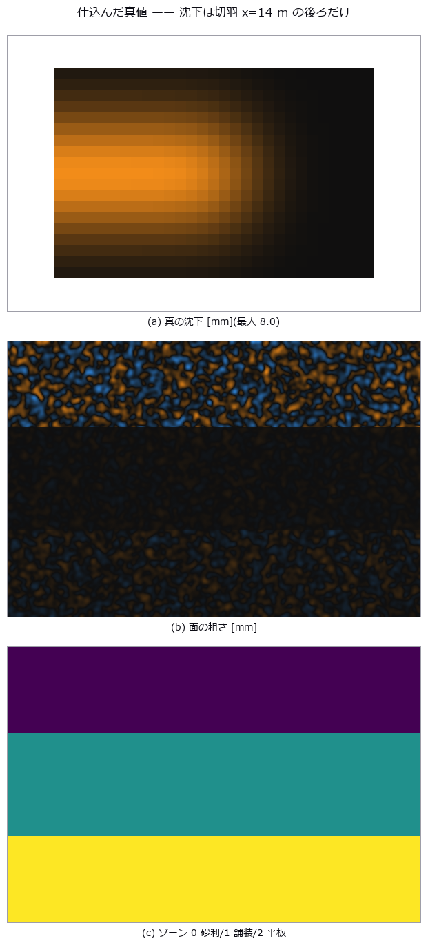
↑ Did It Settle, or Did We Just Scan It Again — What Changes When You Cut at the Detection Limit ―― A 24 x 16 m road surface settling above a tunnel drive, measured from two epochs of point cloud. The nearest-neighbour baseline (C2C) returns a median of 47.74 mm even with zero change — that is just the point spacing — and carries no sign. M3C2 averages -2.43 mm, matching the truth, but only 275 of 551 cores (49.9 %) exceed their level of detection, and those average -4.34 mm: the single averaged number agrees with neither. LoD is a map of the surface, not of the settlement, ranging 0.51 to 3.58 mm across zones. Summing only the significant cores shrinks the volume from 0.8569 to 0.7643 m3, and that shortfall is predictable in advance from the per-core LoD (0.867 predicted versus 0.892 measured).

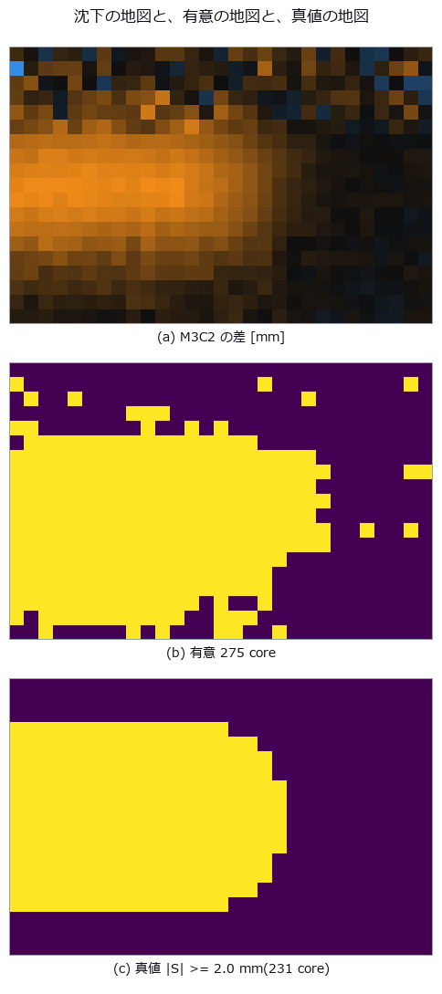
↑ The measurement ―― 有意の地図は真値の地図をよく復元する(TPR 88.7 % / FPR 3.6 %)。ただし縁が痩せる —— そこが 7 節の体積の話。 (figure labels are in Japanese; the numbers are the same)

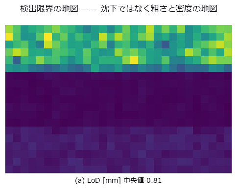
↑ 上の帯(砂利の路肩)は粗さ 15 mm・密度半分なので LoD が跳ね上がる。

↑ 予測は 1.96·σ·sqrt(1/na+1/nb)。

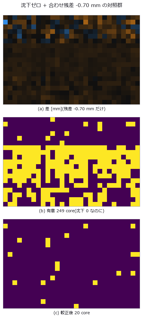
↑ LoD は雑音しか見ていないので、系統誤差はそのまま「有意な沈下」として通る。

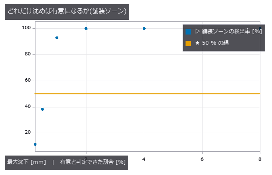
↑ 崖の位置はそのゾーンの LoD で決まる。

py -3.11 examples/poc_settlement_significance.py

Source: examples/poc_settlement_significance.py

This run produced 7 figures in total - see them all

No.2026.041 —— Template Tracking Drifts Quietly Before It Ever Loses the Target

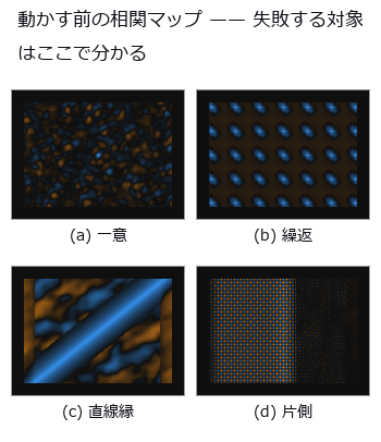
↑ Template Tracking Drifts Quietly Before It Ever Loses the Target ―― A camera moved by a known similarity transform, exposing the three ways template tracking fails: losing the target, drifting quietly, and being confidently wrong. All 152 of the 152 drifted frames passed the peak threshold calibrated without occlusion and reported 'found'. The only absolute quantity measurable without ground truth is forward-backward inconsistency.

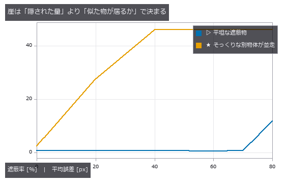
↑ The measurement ―― 同じ遮蔽率でも、そっくりな別物体が視野に居るだけで崖がはるかに手前へ来る。 (figure labels are in Japanese; the numbers are the same)

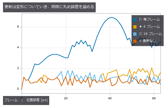
↑ 更新なしは平らなまま。

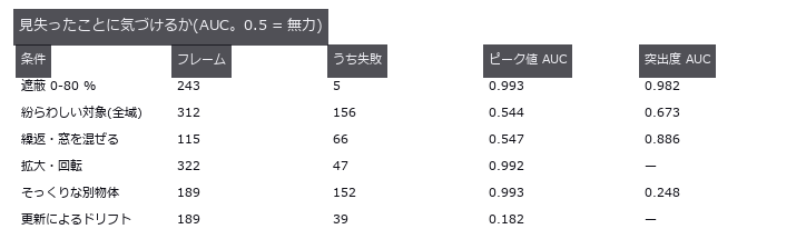
↑ 得意な崖が逆。

py -3.11 examples/poc_template_tracking.py

Source: examples/poc_template_tracking.py

This run produced 4 figures in total - see them all

Ops used (notes): ncc_locate · reflect · shape_locate

No.2026.044 —— A Growth Time-Lapse as Space-Time Connected Components

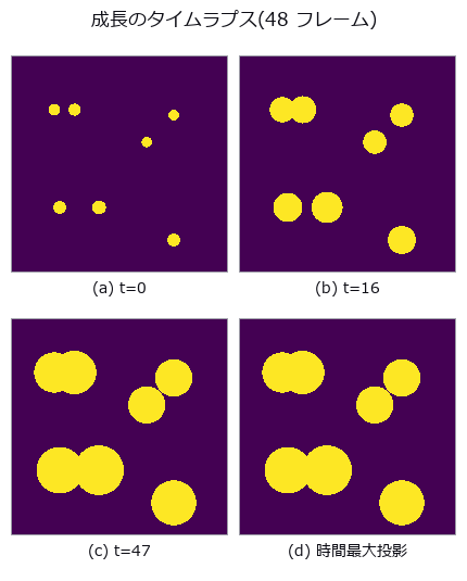
↑ A Growth Time-Lapse as Space-Time Connected Components ―― A video of colonies spreading and merging, read as a (t, y, x) volume with 3-D connected components. Pixel area makes merging look early (-1.16 frames for pair 0-1) while rounding onto the frame grid makes it look late (+0.94); the two oppose, so the sum looks small. The default 26-connectivity of vol_label merged a near miss with a gap of 0.92.

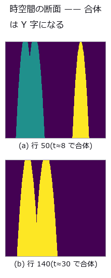
↑ The measurement ―― 縦が時間(下向き、4 倍に拡大)、横が列。2 本の管が合わさる高さがそのまま合体時刻。色は 3-D ラベル。 (figure labels are in Japanese; the numbers are the same)

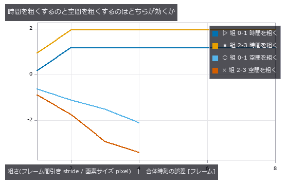
↑ 横軸はどちらも『何倍粗くしたか』。

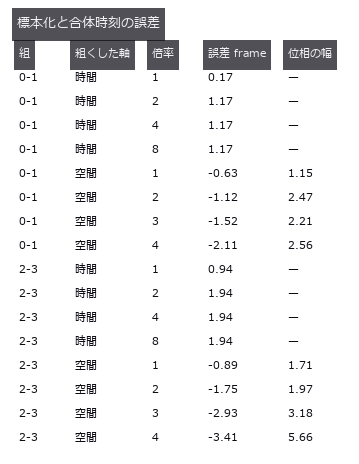
↑ 空間側は格子の位相でこれだけ動く(偏りより大きい)。

py -3.11 examples/poc_timelapse_growth.py

Source: examples/poc_timelapse_growth.py

This run produced 4 figures in total - see them all

Ops used (notes): blob_label · vol_label · vol_region_props

No.2026.045 —— Counting in (x, y, t) — Vehicles Passed, Occlusion, and One Constant: L/V

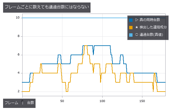
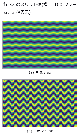
↑ Counting in (x, y, t) — Vehicles Passed, Occlusion, and One Constant: L/V ―― A synthetic traffic video counted per frame, by a virtual loop, and by connected components in a (t, x) slit image. The per-frame maximum reports 7 for 10 vehicles passed — it measures a different quantity. All three failure conditions are written with one constant, vehicle length over speed = L/V (9.0 frames); at a frame interval of 16 the bands fragment and 10 vehicles become 49.

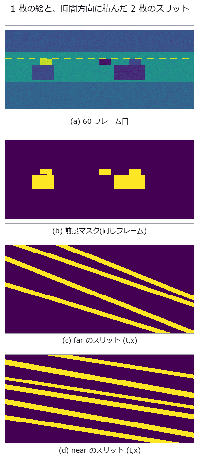
↑ The measurement (figure labels are in Japanese; the numbers are the same)

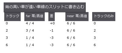
↑ トラックは画像の 50 行から 99 行を占めるので、遠い車線の計数行 63 を横切る。

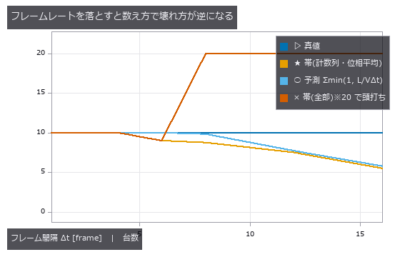
↑ 全部の帯を数えると千切れて過大に(実測は最大 67 だが、他の系列が潰れるので 20 で頭打ちにして描いている)、計数列と交わる帯だけなら見逃しだけ。

py -3.11 examples/poc_traffic_counting.py

Source: examples/poc_traffic_counting.py

This run produced 4 figures in total - see them all

Ops used (notes): blob_features · blob_label · threshold

No.2026.089 —— Where the Warehouse Dwell Came From — Count Waiting Without Its Kind and Everything Is Just Congestion

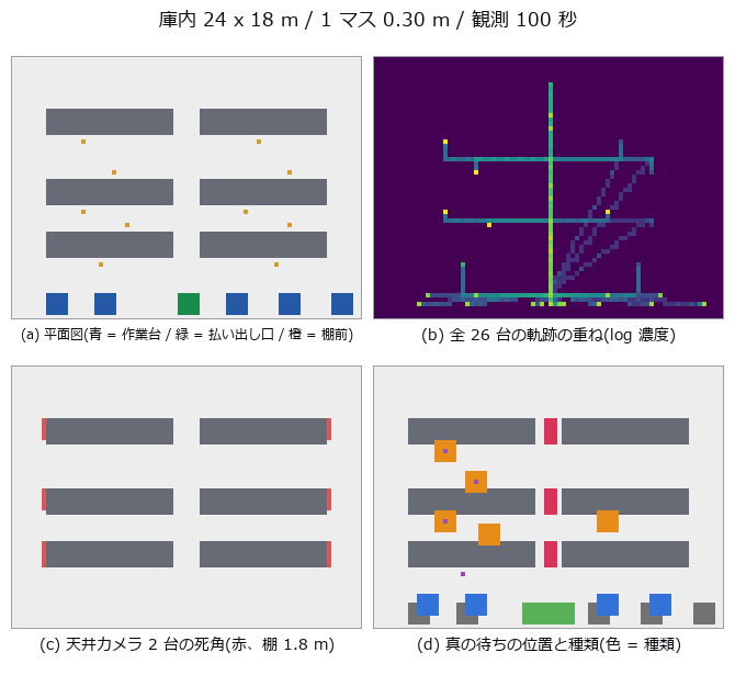
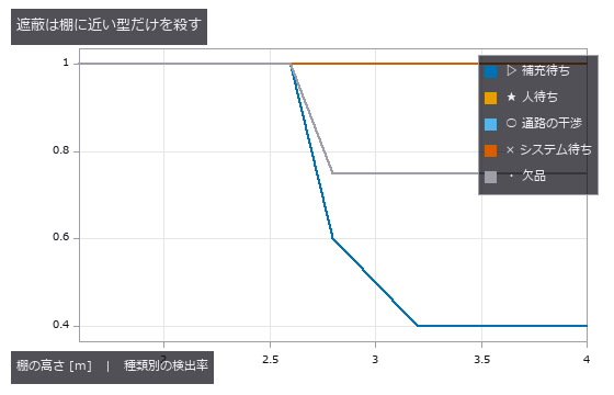
↑ Where the Warehouse Dwell Came From — Count Waiting Without Its Kind and Everything Is Just Congestion ―― A synthetic warehouse floor plan with 26 tracked workers and AGVs, in which replenishment waits, queueing, aisle interference, system waits and stockouts were planted with known times and durations, then read as one (t, y, x) volume. Of the naive 321.5 s of "total dwell", only 198.0 s (61.6 %) is real waiting; the rest is productive work and creep. Removing all queueing or all aisle interference moves that single number by -39.0 s versus -38.0 s, so it cannot say which to fix, while the per-kind counts drop to zero only for the kind that was removed. A stockout moves dwell by -17.0 s but adds 94.6 m of walking, and the three degradation axes each kill a different kind: sampling interval kills the short waits, occlusion kills the waits pressed against racks, and ID merging kills the two kinds defined by a relation between two people.

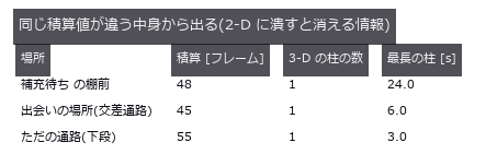
↑ The measurement ―― ヒートマップは場所を当てるが、「1 人が長く待った」と「何人も短く止まった」を分けない。 (figure labels are in Japanese; the numbers are the same)

↑ ゼロ点はこの表を 1 つの数字に畳む。

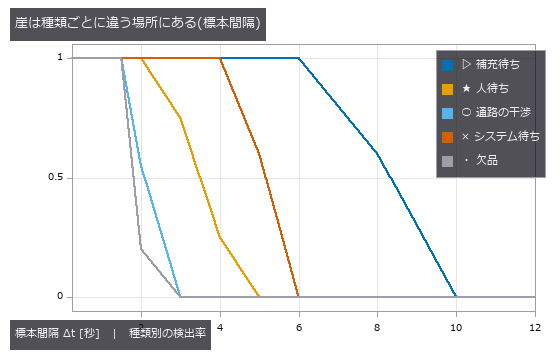
↑ 短い待ち(通路の干渉・欠品)から先に消える。

↑ 天井カメラ 2 台。

↑ 上段は通路が明るい(人が通っただけ)。

py -3.11 examples/poc_warehouse_flow.py

Source: examples/poc_warehouse_flow.py

This run produced 12 figures in total - see them all

Ops used (notes): esdf · face_areas · mesh_volume · occupancy_grid · render_volume_projection · vol_dilate · vol_erode · vol_label · vol_opening_ball · vol_region_props

No.2026.053 —— The Arrival-Time Surface as an Isosurface in (x, y, t)

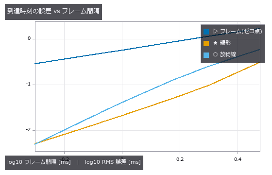
↑ The Arrival-Time Surface as an Isosurface in (x, y, t) ―― The arrival-time surface of wavefronts spreading from point sources, extracted as an isosurface of the (x, y, t) volume. The null (first frame above threshold) is biased by Δt/2, which more frames cannot remove; linear sub-frame interpolation is 27x better (0.0209 ms). Parabolic interpolation loses to linear, and linear is at its best (a 3.8x margin) when the threshold sits at the Gaussian's inflection point θ = 0.6065.

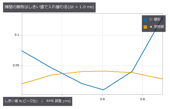
↑ The measurement ―― 変曲点 θ=0.6065 では線形が 3.8 倍勝ち、θ=0.2 では放物線が 3.6 倍勝つ。交点は θ≈0.35 と θ≈0.75。 (figure labels are in Japanese; the numbers are the same)

↑ 各帯の中央値。

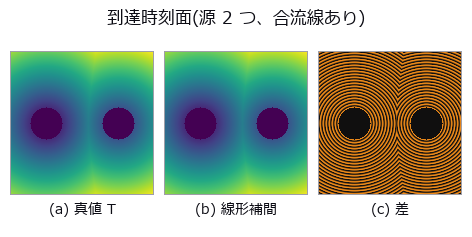
↑ 差は上下 99 % 分位(±0.0327 ms)で切った。

py -3.11 examples/poc_xyt_event_surface.py

Source: examples/poc_xyt_event_surface.py

This run produced 4 figures in total - see them all

Ops used (notes): vertex_normals · vol_edge_probe

No.2026.127 —— A Clip as a Space-Time Cube — What Passed Where, and When, in One Solid

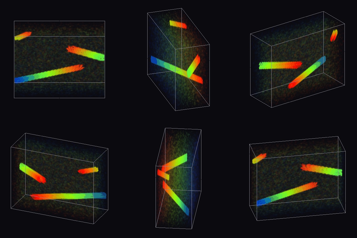
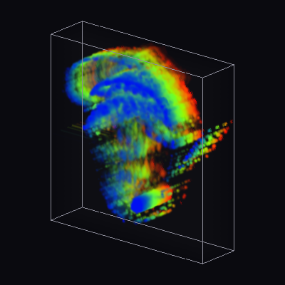
↑ A Clip as a Space-Time Cube — What Passed Where, and When, in One Solid ―― Video Summagator (Nguyen, Niu and Liu, ACM CHI 2012) turns a clip into an (x, y, t) cube, renders the static background faintly and moving objects densely, and lets you cut and rotate the cube to jump to a scene. The new family videocube re-implements it in 6 ops (numpy + scipy only, no new types): frame-difference magnitude as opacity (video_spacetime_cube), front-to-back alpha compositing from any viewpoint with trails coloured by time (blue = start, red = end; vol_render_transfer), cuts (video_cube_cut: x-t slit scans), orbits (video_cube_orbit), keyframes (video_summary_keyframes) and animated GIF export (video_write_gif, the reusable exit). On a synthetic surveillance clip with three objects of known row, onset and speed, the onset read from the first row of each slit-scan streak and the speed read from its slope match the truth exactly (±0 frames; +2.00 / −1.50 / +1.00 px/frame), and the keyframes catch all three onsets (a random choice of 4 frames catches 0.21 on average). The same operators applied to a z-stack of fly-brain EM sections (CREMI sample A, 32 sections, raw data never committed) turn membranes into depth-coloured tubes with neurites running through the stack. In Studio, Tools ▸ Video cube runs it interactively (drag to orbit, slide the cut plane, click the slit scan to jump to that frame, open .npy / GIF / video / .hdf stacks, Save GIF).

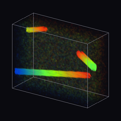
↑ The measurement ―― the clip as a space-time cube (time = depth to the right): moving objects leave trails coloured by time (blue = start, red = end); the static background is a faint grey (figure labels are in Japanese; the numbers are the same)

↑ x-t slit scans of the three rows: a streak's first row is the onset, its slope is the speed (yellow line = injected onset)

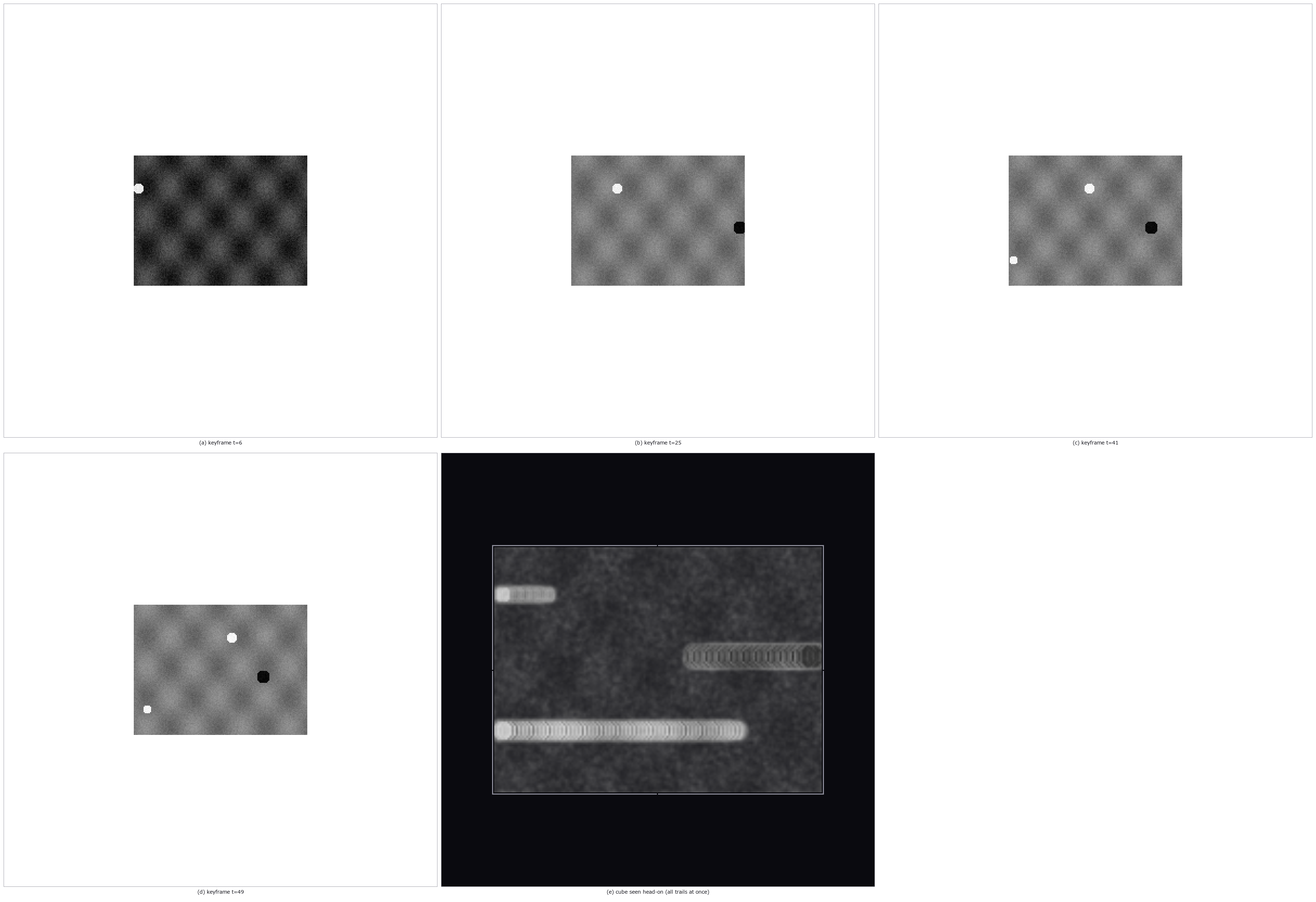
↑ video_summary_keyframes picks the frames right after each object appears; the head-on cube is the whole clip in one image

↑ a real clip from this repo (a turntable GIF, 40 frames of 160x160): a rotating object becomes a helix in the space-time cube

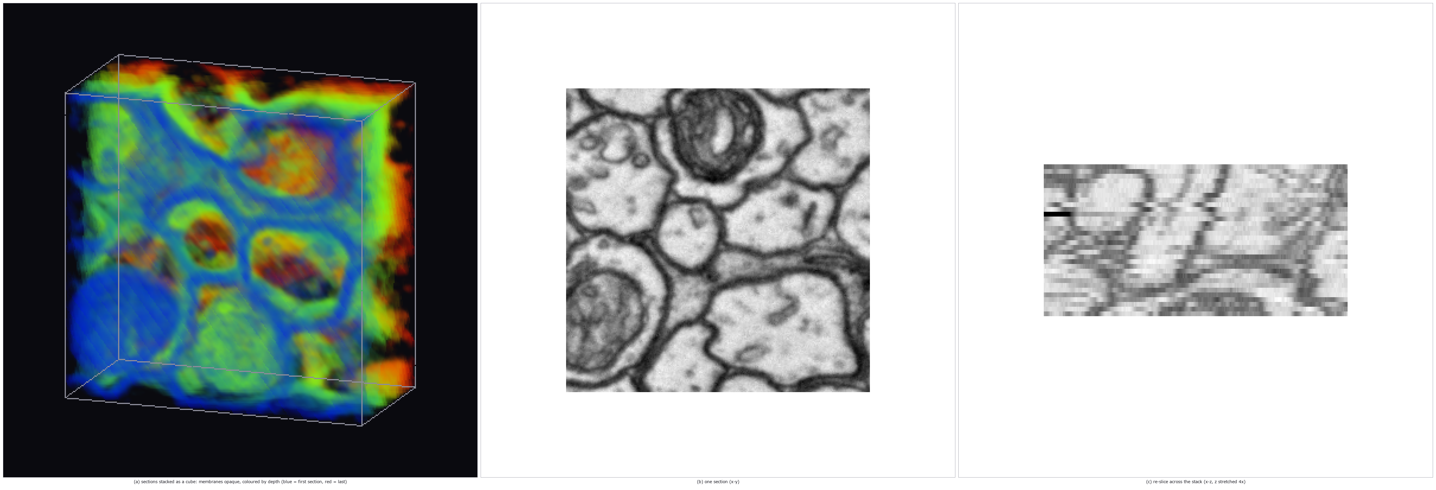
↑ the same cube operators on a z-stack of EM sections (CREMI sample A, 32 sections of 256^2 (adult Drosophila FAFB)): membranes become tubes running thr…

↑ The animation ―― the EM stack rotating: neurites are the tubes, coloured by depth; the same operator that rotated the surveillance clip

py -3.11 examples/poc_video_cube.py

Source: examples/poc_video_cube.py

This run produced 7 figures in total - see them all

Ops used (notes): intensity · video_cube_cut · video_cube_orbit · video_spacetime_cube · video_summary_keyframes · video_write_gif · vol_render_transfer

No.2026.128 —— Living Tissue in 3D+t Without a Generator — Magnify, Flow, Interpolate, Height, All Against Truth

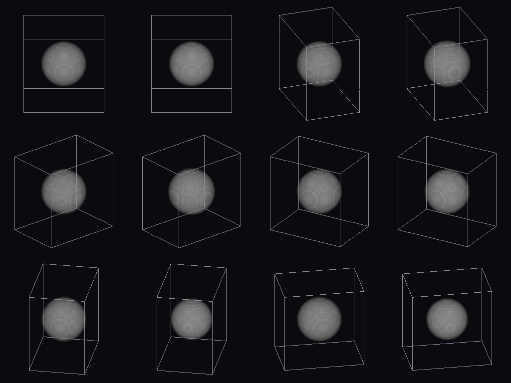
↑ Living Tissue in 3D+t Without a Generator — Magnify, Flow, Interpolate, Height, All Against Truth ―― A video generator invents plausible motion. The new family live4d (14 ops, numpy + scipy only, one new word: volseq = a volume series (T, Z, Y, X)) invents nothing; instead it offers four ways to make real motion visible, each pinned to numbers on synthetic series with known truth. (1) Magnify: a shell whose radius beats by 0.1 voxel (invisible) is magnified x8 by volseq_magnify_motion (a 3-D version of Wu et al.'s linear Eulerian magnification); the radius amplitude read back is 7.89 x and the period is unchanged. (2) Flow: the displacement field of two blobs separating at a known ±0.75 voxel/frame (vol_flow_3d, 3-D Lucas–Kanade) reads +0.776 / −0.776 where there is gradient, and the pathlines (volseq_pathline_render) become one solid coloured by time. (3) Interpolate: a series made at twice the rate, halved and refilled by volseq_interpolate_flow, matches the removed frames with RMSE 0.0016 when the motion per step is twice the blob size (a linear blend: 0.0207) — while below about 0.8 sigma per step the blend is as good and the warp's resampling costs a little (plotted honestly). (4) Height: from a focus-sweep series (a moving bump) focus_sweep_height_video recovers the height field with RMSE 0.31 planes. Live cells in 3D+t from the Cell Tracking Challenge (Fluo-N3DH-CHO, raw data never committed) run through the same path.

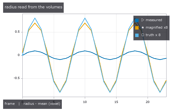
↑ The measurement ―― radius of the shell read from each volume: the measured beat (0.10 voxel) is below one voxel; after magnification it follows alpha x truth (figure labels are in Japanese; the numbers are the same)

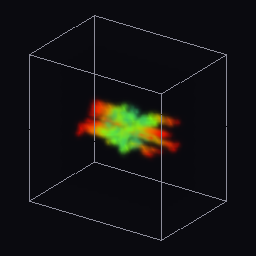
↑ pathlines of particles carried by the 3-D flow of the dividing blob, coloured by time (blue = start, red = end); the faint grey is the first volume

↑ a frame removed from a 2x-rate series (motion 5 voxel = 2 sigma per step) re-created two ways (max projections): the linear blend shows two ghosts per…

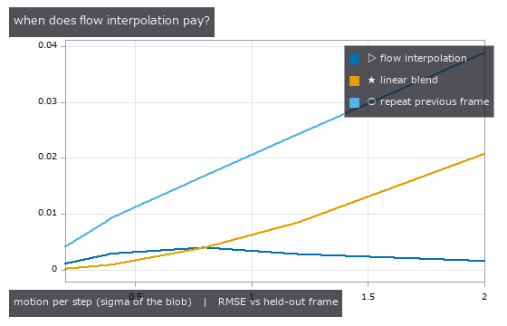
↑ error of the re-created frames against the removed ones, as the motion per step grows: below about one blob width a linear blend is as good (the warp'…

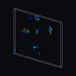
↑ Fluo-N3DH-CHO/01 (12 volumes of (5, 111, 128), y/x 1/4): pathlines of the 3-D flow between consecutive volumes, coloured by time

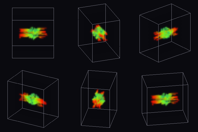
↑ The animation ―― the same pathlines orbited: two straight bundles leaving the split point at +/-0.75 voxel/frame

↑ The animation ―― height field recovered from a focus sweep series (a moving bump, 11 planes), shaded and coloured by height (blue = low, red = high); RMSE 0.31 planes

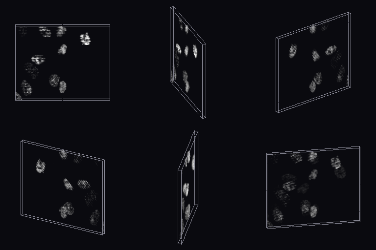
↑ The animation ―― Fluo-N3DH-CHO/01 (12 volumes of (5, 111, 128), y/x 1/4): the live volumes orbited while time advances (intensity as opacity)

py -3.11 examples/poc_live4d.py

Source: examples/poc_live4d.py

This run produced 10 figures in total - see them all

Ops used (notes): blend · focus_sweep_height_video · focus_sweep_surface_video · vol_flow_3d · volseq_interpolate_flow · volseq_magnify_motion · volseq_pathline_orbit · volseq_pathline_render · volseq_render_orbit · volseq_synth_beating · volseq_synth_dividing

No.2026.145 —— Testing the Periodic Boundary of Temporal Operators with a Seamless Loop

↑ Testing the Periodic Boundary of Temporal Operators with a Seamless Loop ―― Periodic material carries an exact invariant that any temporal operator must satisfy: for a video of period T, an operator that handles the periodic boundary correctly obeys op(roll(v,k)) == roll(op(v),k) exactly, and any implementation that pads the ends by replication, clamping or truncation breaks it. Because perpetual_loop makes every time-dependent quantity a function of theta, the seam is never created rather than removed (seam ratio 1.0509, where 1 and not 0 is the correct answer), so the truth for that equality is exactly zero difference. No new operator was added. The core finding is that a perfect score came out of an empty output: run with its defaults, three_frame_difference reports a maximum difference of 0.0e+00 and zero contaminated frames, yet only 0 of 32 frames carry any content - the default threshold of 0.1 exceeds the material's largest frame-to-frame change of 0.0841, so nothing is detected at all, and an empty output shifts to another empty output, agreeing trivially. Lowering the threshold to 0.03 gives the same operator 30 of 32 frames of content, 4 contaminated frames and a maximum difference of 1.000 - the perfect score was a lie. Scanning all sixteen single-input video-to-video operators in the ledger splits them into three groups: windowed operators contaminate only the ends (2 frames for causal frame differencing and optical-flow magnitude, 4 for the moving average, 8 for windowed background subtraction, temporal bilateral and temporal median), so trimming that many frames leaves the rest exactly equivariant; recursive or globally normalising operators contaminate all 32 frames and trimming does not help; and three operators return almost nothing, which reads as zero contamination but is not a pass. The contaminated frames are predictable not merely in count but as a set: a window of width w contaminates roll(B,k) union B, and across w = 3, 5, 7, 9, 11 and 13 the predicted set matched exactly (4, 8, 12, 16, 19, 21). The naive prediction of w-1 frames fails in all six cases and 2(w-1) fails at w = 11, where the two bands overlap by exactly one frame at T = 32 with a shift of 9. The first prediction assumed a centred window and was wrong; subtracting the mismatched sets showed contamination only at the head with the tail untouched, which means the window is trailing rather than centred - the orientation of a window can be read off the shape of the contaminated set without reading the implementation.

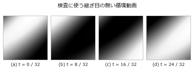
↑ The measurement ―― perpetual_loop("plasma_orbit") の 4 コマ。時間に依る量をすべて θ の関数にしてあるので、t = T は t = 0 と同じ式です ---- 継ぎ目は消したのではなく最初から作られていません(継ぎ目の比 1.0509、0 ではなく 1 が正解)。★だから「巡回シフトしても同じ動画」という厳密な真値が素材の側に立ちます。 (figure labels are in Japanese; the numbers are the same)

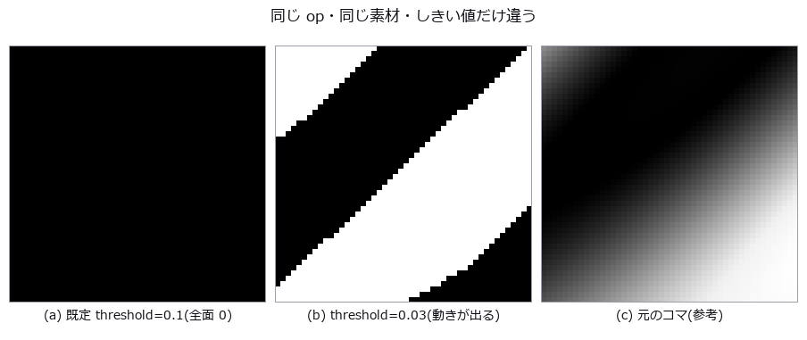
↑ three_frame_difference の同じコマです。

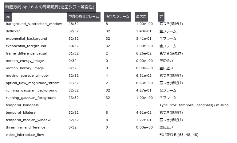
↑ 継ぎ目の無い動画 32 コマを巡回シフトして測った全数走査です。

↑ 窓幅 7 のときに汚れたフレームの位置。

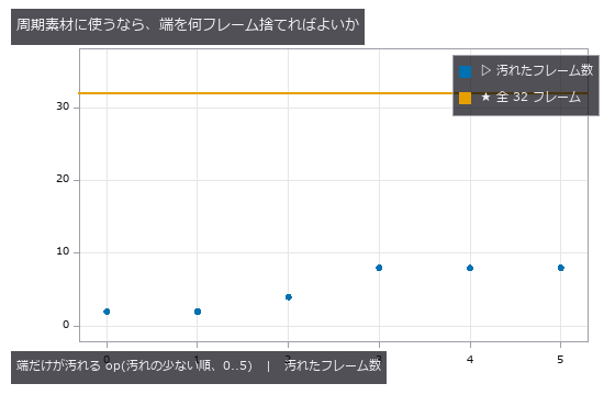
↑ 端だけが汚れる 6 本について、汚れたフレーム数を少ない順に並べたもの。

↑ The animation ―― 同じ動画を実際に回したもの(32 コマ)。最後のコマから最初のコマへ戻るところに継ぎ目が見えません ---- 消したのではなく、時間に依る量をすべて θ の関数にしてあるので最初から存在しないからです。★この性質があるので「巡回シフトしても同じ動画」が厳密な真値になり、時間方向 op の周期境界を数で採点できます。

py -3.11 examples/poc_periodic_video_boundary.py

Source: examples/poc_periodic_video_boundary.py

This run produced 9 figures in total - see them all

Ops used (notes): moving_average_window · perpetual_loop · perpetual_loop_seam · three_frame_difference

The Geometry and Calibration Wing — A Small Residual Is Not Proof of Correctness

Reprojection error in camera calibration, seam mismatch in a panorama, residual in point-cloud registration: all are read as 'smaller is better'. The 7 exhibits here, with ground truth in hand, show where that reading fails.

Reprojection RMS of 0.0688–0.0690 px alongside focal-length errors of 0.026–7.334 %. Adjacent seams at 0.12 px while the single closing seam opens by 1.5 px. Spheres and cylinders converging to the same residual with an arbitrary pose. Least squares drives the residual down to the noise; whether it lands on the truth is a separate question.

A trap in the measuring procedure itself is kept on display: fix one point cloud and sweep only the pose, and you still have a sample of one — the random seed alone produced both '0 % quadrant errors' and '100 %'. About the only absolute quantity measurable without ground truth is the loop-closure error of a full 360-degree sweep.

No.2026.006 —— A Reprojection Error of 0.05 px Guarantees Nothing

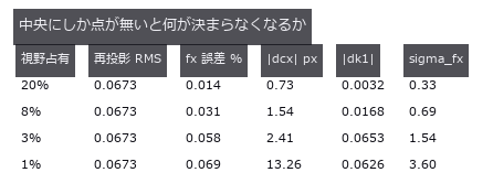
↑ A Reprojection Error of 0.05 px Guarantees Nothing ―― Grid points projected with known intrinsics and poses, re-calibrated, and the error split by component. With the board tilted 32 / 8 / 2 degrees the reprojection RMS spans 0.0688 to 0.0690 px (ratio 1.00) while the focal-length error spans 0.026 to 7.334 % (281x). With a distorting camera the degeneracy gate never fires, and the non-linear optimiser returns an answer even for a fronto-parallel board.

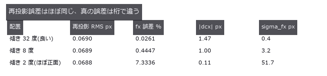
↑ The measurement ―― RMS は 1.00 倍しか動かないのに fx 誤差は 281 倍動く。配置の良し悪しを映すのは sigma_fx のほう。 (figure labels are in Japanese; the numbers are the same)

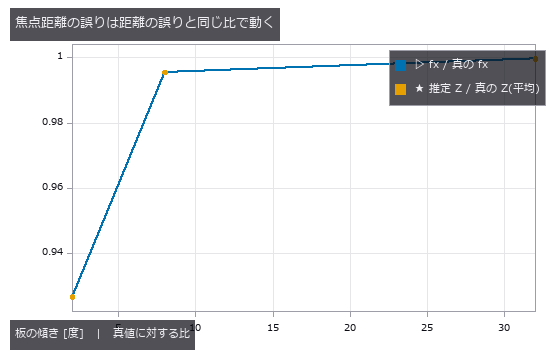
↑ 2 本は重なる。

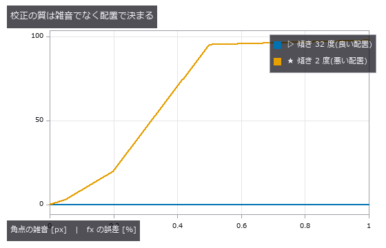
↑ どちらも雑音 0 では真値。

py -3.11 examples/poc_camera_calibration.py

Source: examples/poc_camera_calibration.py

This run produced 4 figures in total - see them all

Ops used (notes): project_points · reprojection_error

No.2026.028 —— Chain the Neighbours Together and You Cannot Get Back Where You Started

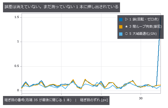
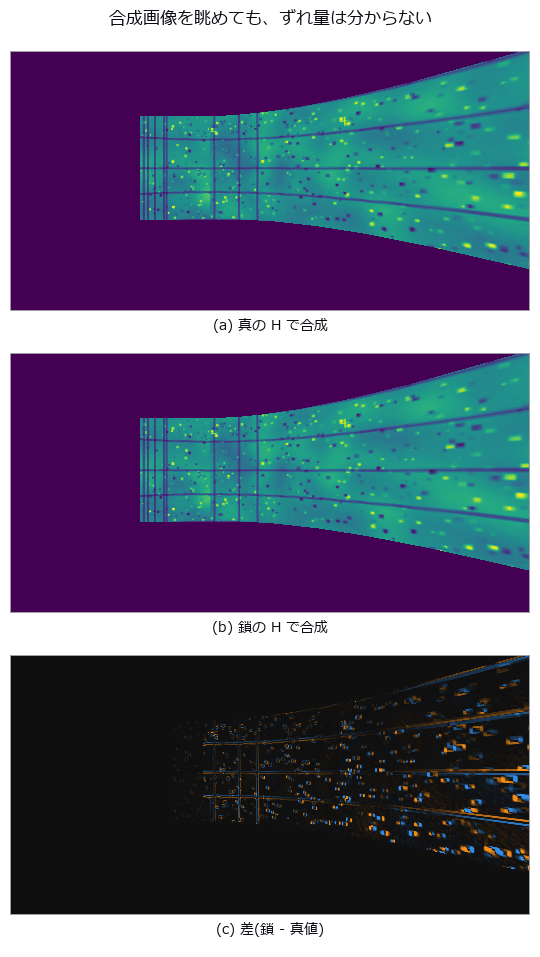
↑ Chain the Neighbours Together and You Cannot Get Back Where You Started ―― 36 frames cut from a cylindrical panorama by a known rotation sequence and chained pairwise around a full turn. Adjacent seams agree to 0.12 px, yet the one closing seam opens by 1.5 px (13x). The buried bundle_adjust_mosaic did not beat the chain (30 of 36 frames were left as the identity); the worst pose error goes from 1.65 px for the chain to 0.56 px with global optimisation.

↑ The measurement ―― 系 2(等分)は閉ループ誤差を下げるのに姿勢はかえって悪化する。新しい観測を足さずに効くのは系 3。 (figure labels are in Japanese; the numbers are the same)

↑ 上 2 枚はどちらも継ぎ目が綺麗に見える(後勝ちの上書きで混合しないため)。

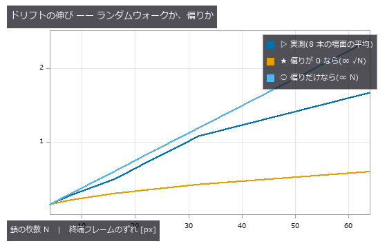
↑ 実測 log-log 傾き 0.89。

py -3.11 examples/poc_panorama_drift.py

Source: examples/poc_panorama_drift.py

This run produced 4 figures in total - see them all

Ops used (notes): pose_error · warp_by_plane

No.2026.108 —— Measuring on a Real Stereo Photograph — Three Stumbles Synthesis Never Produces

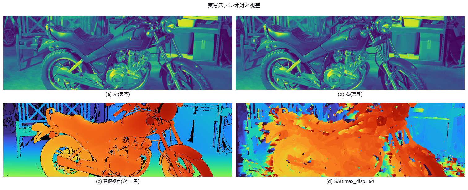
↑ Measuring on a Real Stereo Photograph — Three Stumbles Synthesis Never Produces ―― The first exhibit in this museum measured on a real photograph (Middlebury 2014 motorcycle, with ground-truth disparity). The distributor's own note says the holes in the truth are NaN; they are +inf, so np.nanmedian reports a median disparity of 44.97 px instead of 42.55 px, while fill_disparity and apply_cmap — which test with isfinite — handle them correctly. The default max_disp=16 scores bad2 95.06 %: any search range below the true maximum of 59.91 px loses the whole foreground, so the cliff sits between 48 and 64, which geometry predicts before any measurement. Against a 94.04 % null, SGM scores 15.81 %, and discarding the least confident 40 % takes it to 6.80 %. Converting to metric depth bends the scene: depth_from_disparity had no principal-point offset, and ignoring the real doffs of 31.086 px puts points 1.519 to 5.243 times too far — no single scale repairs it, since the best factor of 0.3733 still leaves 958.3 mm RMS over a 2889 mm range, pushing far surfaces +1676 mm out and pulling near ones -926 mm in. The argument was added here, and it reproduces the closed form exactly.

↑ The measurement ―― 下位 4 割を捨てると bad2 は 26.75 % -> 6.80 %。 (figure labels are in Japanese; the numbers are the same)

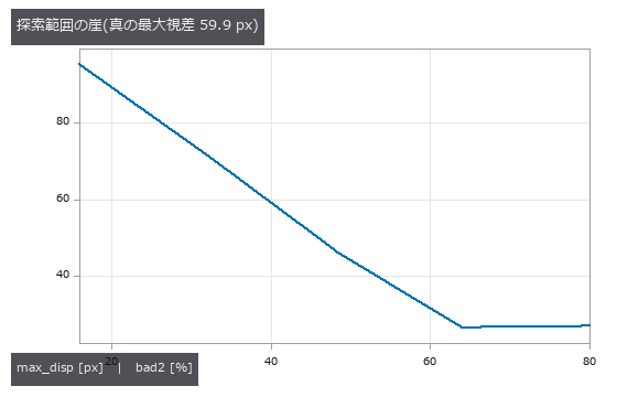
↑ 真の最大視差を下回る設定は前景を丸ごと失う。

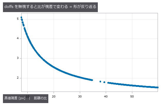
↑ 単一のスケールでは直らない(最良でも残差 958 mm RMS)。

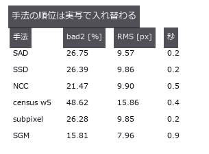
↑ census が最下位なのは窓が 64 bit で頭打ちだから。

py -3.11 examples/poc_real_stereo_depth.py

Source: examples/poc_real_stereo_depth.py

This run produced 5 figures in total - see them all

No.2026.034 —— The Convergence Basin of Point-Cloud Registration — How Far Off Can the Initial Pose Be?

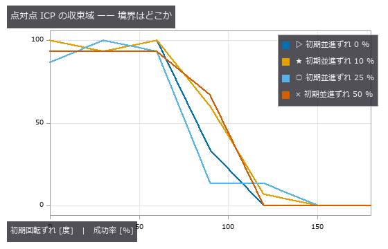
↑ The Convergence Basin of Point-Cloud Registration — How Far Off Can the Initial Pose Be? ―― ICP success rate contoured against the initial pose error, with the point cloud re-sampled on every trial. With no translation offset, success drops below 50 % at 90 degrees for point-to-point and 120 degrees for point-to-plane. Spheres and cylinders converge to the same residual with an arbitrary pose; with the global method all 16 of 16 trials appear converged and the pose is wrong — undetectable from the residual.

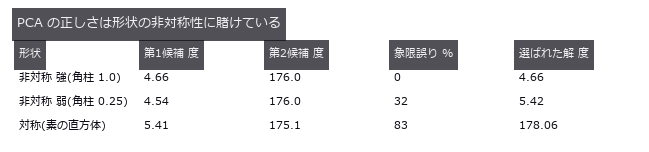
↑ The measurement ―― 非対称性が消えると 4 候補が形として区別できず、選択が崩れる(選ばれた解が第 1 候補から離れる)。 (figure labels are in Japanese; the numbers are the same)

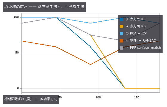
↑ 平らな線ほど「広い」。

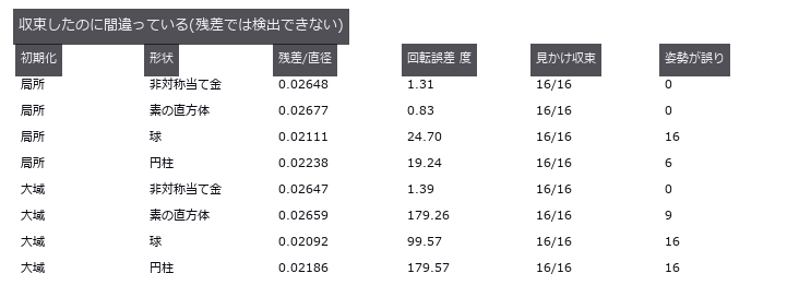
↑ 球・円柱は残差が小さいまま姿勢が任意。

py -3.11 examples/poc_registration_basin.py

Source: examples/poc_registration_basin.py

This run produced 4 figures in total - see them all

Ops used (notes): estimate_normals · farthest_point_sampling

No.2026.117 —— Which Quantities Really Survive a Rotation — Auditing Invariance on a Real Coin

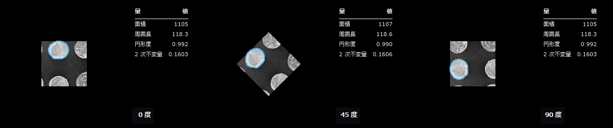
↑ Which Quantities Really Survive a Rotation — Auditing Invariance on a Real Coin ―― Shape features are routinely called rotation-invariant, but the pixel grid is not invariant under rotation, so the claim usually breaks at a helper — how the boundary is counted, how the image is interpolated, where the threshold lands. A real photograph (scikit-image coins, Greek coins from Pompeii, British Museum) is turned through a full circle in 5-degree steps and the wobble is split into three arms: A rotate the greyscale and re-threshold (what people actually do), B rotate the 0-degree binary mask with nearest neighbour (re-rasterisation only), C multiples of 90 degrees via np.rot90 (exact). The rotation itself is done with scipy, not with fullseye — measuring your own invariance with your own rotation hides errors that lean the same way. Arm C is exactly 0.00 % for all seven quantities: the measurements carry no orientation bias at all, so every bit of the wobble is the cost of re-laying the boundary on the grid. The prediction was wrong: rotating the binary mask turns out to be far worse than interpolating the grey — perimeter 2.52 % (A) vs 9.47 % (B), circularity 4.82 % vs 20.45 %. Nearest-neighbour rotation re-lays a staircase; interpolating the grey re-derives the boundary from the underlying continuous signal. Rotate the greyscale, never the mask. A synthetic square anchors the closed form: the 4-connected staircase perimeter of a square rotated 45 degrees is bounded by 4L → 4L√2 (+41.4 %), but the measured swing is 7.91 % because regionprops applies a Crofton-style correction — the closed form is a ceiling, not a prediction. Finally, check the denominator: Hu[1] is ~0 for a near-circular blob (3.9e-04), so its 29.6 % relative spread means nothing at all.

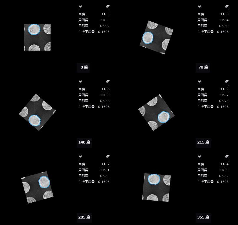
↑ The measurement ―― 実写の硬貨を 5 度ずつ 1 周。地がモノクロなので輪郭は彩度のある色で描いている(灰色には彩度が無いので、どの階調とも色相で区別がつく)。右の表の数字がどれだけ揺れるかが見える。 (figure labels are in Japanese; the numbers are the same)

py -3.11 examples/poc_rotation_invariance_audit.py

Source: examples/poc_rotation_invariance_audit.py

This run produced 2 figures in total - see them all

Ops used (notes): annotate_outline · annotate_table · blob_features · blob_label · circularity · eccentricity · moments_region_2nd_invar · moments_region_central_invar · text_box

No.2026.133 —— Where Is the Public Camera Looking — The Orientation of a Fixed Camera Whose Only Published Fact Is Its Position, from the Picture Itself

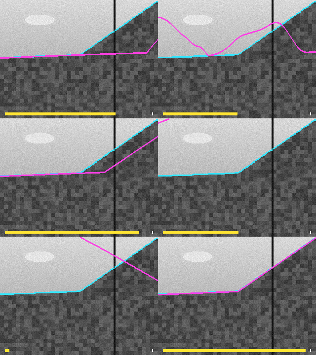
↑ Where Is the Public Camera Looking — The Orientation of a Fixed Camera Whose Only Published Fact Is Its Position, from the Picture Itself ―― Public fixed cameras (road, weather, tourism) publish their position but not their orientation, or only a coarse one (a road direction code, an id hash, a manual gizmo); without the orientation a frame cannot be placed on a map, a DEM or a 3-D city. The new geocam family (7 ops, numpy + scipy) recovers the (yaw, pitch, roll) of a camera at a known position from the picture itself, with no learning, from two independent cues that check each other. (1) Skyline: the 360-degree ridge rendered from a DEM at the camera position (dem_skyline, with earth curvature and refraction and the horizon dip as the floor outside the DEM) is matched against the sky/terrain boundary extracted by dynamic programming (skyline_extract, Lie et al. 2005); camera_orientation_from_skyline returns the whole residual curve over yaw and the margin to the runner-up valley. (2) Sun: the apparent sun position is a closed form of time and place (sun_position, NOAA, checked against equinox and solstice values); two or more saturated sun discs picked from time-stamped frames (sun_pixel_position, which refuses clouds and sky bands by their fill ratio) fix the rotation exactly as the SVD solution of Wahba's problem (camera_orientation_from_sun). On a synthetic camera with a known pose (synthetic DEM, sky, a cloud, a foreground pole, noise, known intrinsics) the skyline route errs by 0.11 / 0.06 / 0.06 deg, the sun route by 0.02 / 0.04 / 0.05 deg (6 frames; the morning and evening frame alone give 0.004 deg), and the two routes agree to 0.09 deg. Controls: a road-direction prior of the kind public metadata gives is off by 7.5 deg, and on a flat DEM the ridge is the same in every direction so the op returns ambiguous instead of being silently 137 deg wrong. Prior work: Lalonde et al. IJCV 2010 (sun and sky, 3 deg on 22 webcams) and Baatz et al. ECCV 2012 (skylines, the large-scale position-unknown version). Honest breakdown: synthetic only (real data - Fintraffic weather cameras + NLS elevation in Finland, Statens vegvesen + Kartverket DTM10 in Norway - is the next step and raw frames are never committed), the intrinsics K are required (an error in K turns into pitch and roll), skylines need mountains and the sun needs to be in the picture.

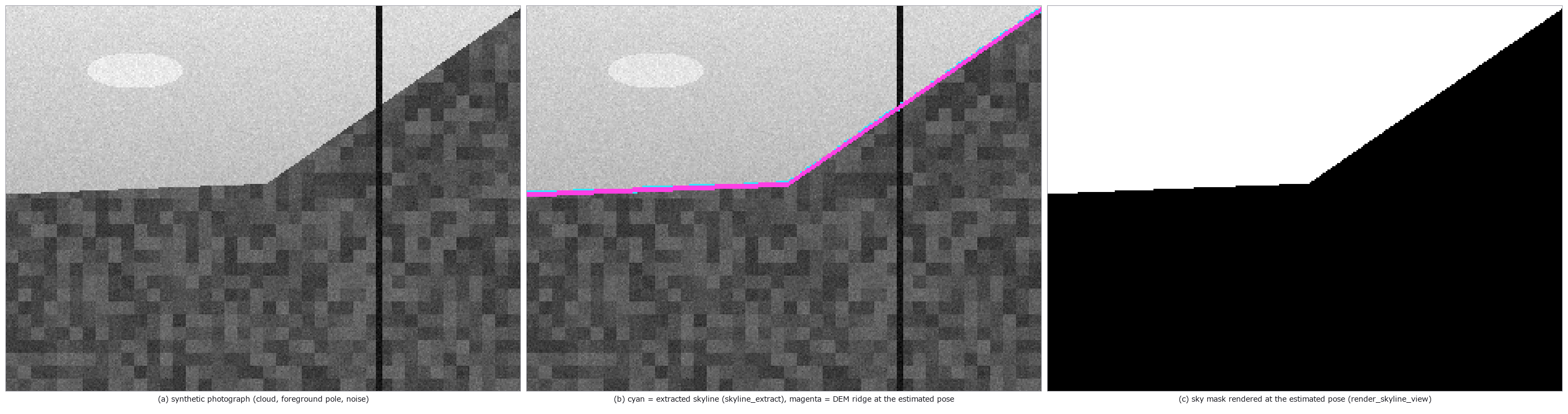
↑ The measurement ―― the DEM ridge drawn at the estimated yaw / pitch / roll lies on the extracted skyline; errors 0.06 / 0.03 / 0.01 deg (figure labels are in Japanese; the numbers are the same)

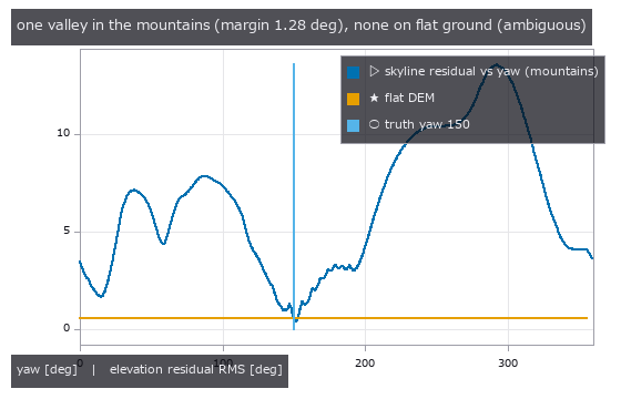
↑ the op returns the whole residual curve so that the ambiguity is visible: a runner-up valley at 15 deg is 1.28 deg worse; the flat DEM curve is level

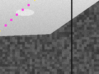
↑ the sun's path over the day where it is above the ridge (yellow, projected with the pose estimated from the sun) and the 5 sun discs picked by sun_pix…

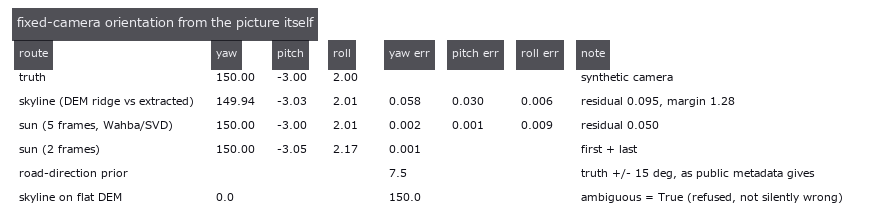
↑ both routes recover the pose to well under a degree and agree with each other; the public-metadata prior is off by ten degrees and the flat-ground cas…

py -3.11 examples/poc_public_camera_heading.py

Source: examples/poc_public_camera_heading.py

This run produced 5 figures in total - see them all

Ops used (notes): camera_orientation_from_skyline · camera_orientation_from_sun · dem_skyline · project · render_skyline_view · skyline_extract · sun_pixel_position · sun_position

No.2026.134 —— Where Is the Public Camera Looking, for Real — Hunting the Sun in 807 Road Cameras, Fixing the Heading from One Sunset and Checking It Against the Road

↑ Where Is the Public Camera Looking, for Real — Hunting the Sun in 807 Road Cameras, Fixing the Heading from One Sunset and Checking It Against the Road ―― The synthetic PoC (poc_public_camera_heading) got away with 'the sun is a small saturated disc'; real road cameras did not. Probing the 24 hours of 20-21 September from Finland's 807 Fintraffic weather cameras (CC BY 4.0, no key) at sun elevations of 2-12 degrees, the look-alone gate (sun_pixel_position) called station-name text, signs, white cars and lens droplets the sun (24/24 wrong on the first probe), the sun is not a disc but a bloom whose size depends on exposure and which the station-name band clips, and the cameras look down at the road with sky in the top third only. Two ops were added to geocam: sun_bloom_fit (a Kasa circle fitted to the unclipped rim of the largest saturated blob; the centroid sits 12 px off on average, away from the cut) and camera_orientation_from_sun_candidates (RANSAC over per-frame candidates for the one blob that moves at the sun's rate in a fixed camera, with road-camera priors |roll| <= 12 deg, pitch -40..0 deg, HFOV 25-120 deg rejecting unphysical hypotheses, the focal length searched at the same time, and no votes from below-horizon times). Over 807 stations x 24 h exactly one sunset could be tracked (E18, Hamina; official metadata says direction UNKNOWN): from 5 frames (15:01-16:01 UTC) yaw 267.9, pitch -4.6, roll 0.9 deg, f 1439 px (HFOV 48 deg), residual 0.34 deg. Independent check: the lane vanishing point (medoid over several daytime frames) turned into a world bearing with the same pose is 272.7 deg against 275.3 deg for the E18 segment in OpenStreetMap - 2.5 deg apart. The weak degrees of freedom are not hidden: under leave-one-out yaw moves 1.3 deg but roll 10 deg and f 2 % (the limit of a one-hour low-elevation arc). On the same frames the look-alone gate said 'sun' 22 times: 3 exact, 2 on the sun but off-centre, 17 something else. Raw frames are never committed; only the aggregate (times, circle fits, vanishing point, road bearing) ships. Sources: Fintraffic / Digitraffic (CC BY 4.0), OpenStreetMap (ODbL).

↑ The measurement ―― the sunset seen by C0362200 (E18, Hamina, Finland; metadata says direction UNKNOWN): the sun's path for the evening drawn from the fitted pose (magenta) and the 5 blooms fitted with a circle (cyan); yaw 267.9, pitch -4.6, roll 0.9, HFOV 48 (figure labels are in Japanese; the numbers are the same)

↑ what the look-alone detector (sun_pixel_position, built for synthetic discs) called the sun in the same camera: 22 picks, 3 exactly the sun, 2 on the…

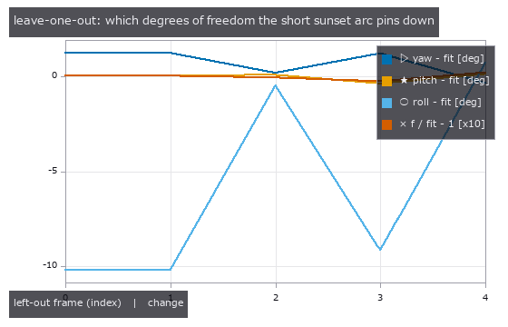
↑ refit with each sun frame removed: yaw barely moves, roll and the focal length are the weak directions of a 1-hour low-elevation arc — this is why the…

↑ for blooms cut by the station-name band the centroid sits 12.4 px (mean) away from the circle fitted to the unclipped rim; the fit uses the circle

↑ one camera out of 807 stations gave a sun track of 4 or more frames on 2026-09-20/21 (2 more had 3 frames and were left out); the vanishing point of i…

py -3.11 examples/poc_public_camera_heading_real.py

Source: examples/poc_public_camera_heading_real.py

This run produced 6 figures in total - see them all

Ops used (notes): bloom · camera_orientation_from_sun_candidates · ellipse · project · sun_position

The Colour and Separation Wing — There Is No Method That Works, Only Conditions Under Which One Does

Estimating the illuminant to restore colour, peeling the layers of a painting with multiple wavelengths, separating specular reflection with polarisation. The 4 exhibits here synthesise linear radiance from known spectral reflectances, known illuminants and the Fresnel equations, then compare the separation against that truth.

The conclusion in every case was that the failure axes are orthogonal. Max-RGB is best when a white patch is present and gets 8x worse when the single brightest patch is removed; grey-world shrugs off saturation but loses once chromatic content exceeds 20 %; under a reference illuminant every method loses to doing nothing; adding bands does not win, adding near-infrared does.

The shared warning is to convert to linear radiance before calling anything. Pass sRGB-gamma values and no exception is raised; the separation simply degrades in silence. Failure without an exception is the most common pattern in the whole museum.

No.2026.032 —— Peeling Layers With Many Wavelengths — Underdrawing, Ground, Glaze and Fading, Truth in Hand

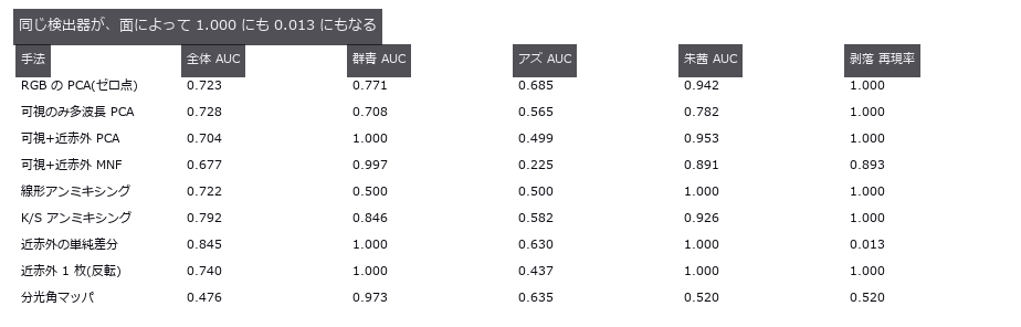
↑ Peeling Layers With Many Wavelengths — Underdrawing, Ground, Glaze and Fading, Truth in Hand ―― A spectral cube of ground, underdrawing, glaze and fading stacked in layers, then unmixed. Splitting the visible range into 16 bands does no better than RGB (recall 0.118 versus 0.119); what won was adding near-infrared. The same detector scores an AUC of 1.000 on ultramarine, 0.630 on azurite and 0.013 on losses — averaged, all of that vanishes. Restoring the unfaded colour barely beat the null, ΔE00 16.79 → 16.46.

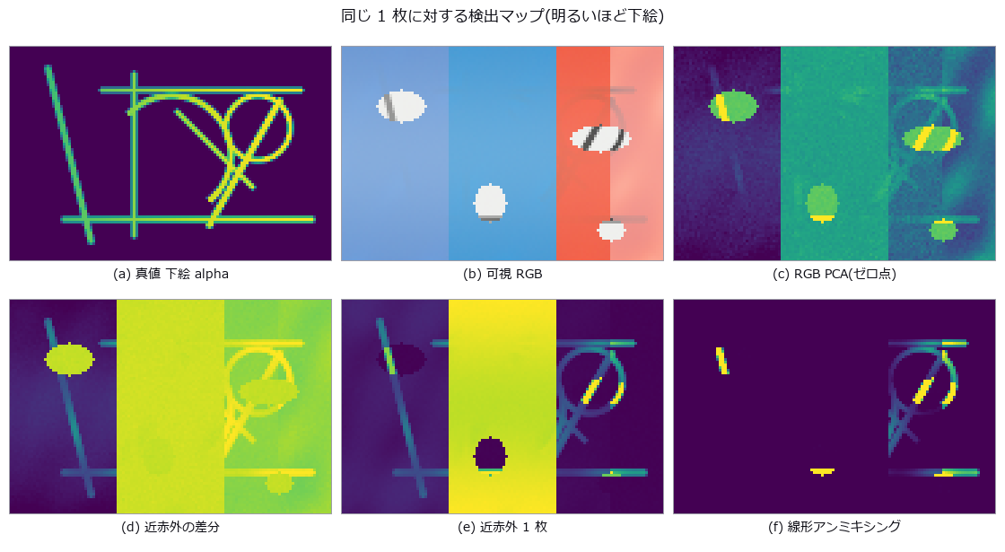
↑ The measurement ―― 近赤外の差分は剥落部(楕円)で消え、近赤外 1 枚は面ごとに水準が違う。塗り分けは 1–99 分位でクリップした表示のみ。 (figure labels are in Japanese; the numbers are the same)

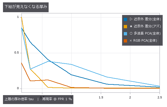
↑ 半分を割るのは tau 0.30–0.60 のあいだ。

↑ ゼロ点の線より下に来た復元が 1 本も無い。

py -3.11 examples/poc_pigment_unmixing.py

Source: examples/poc_pigment_unmixing.py

This run produced 4 figures in total - see them all

Ops used (notes): delta_e_map · linear_to_srgb · spectrum_to_srgb · threshold

No.2026.033 —— Stripping Specular Reflection With Polarisation — Truth From the Fresnel Equations

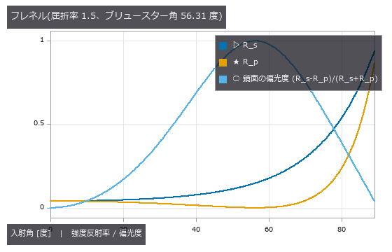
↑ Stripping Specular Reflection With Polarisation — Truth From the Fresnel Equations ―― Diffuse and specular components synthesised as s/p terms with the degree of polarisation from the Fresnel equations, and the separation scored against them. At 20 degrees of incidence the polarisation method wins by only 1.2x. The diffuse error matches the closed form R_p·E exactly and vanishes at the Brewster angle of 56.31 degrees — the diffuse term of polarization_separate is systematically high by that amount.

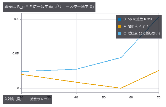
↑ The measurement ―― 実測と閉形式が重なる。70 度の絶対誤差は 20 度より悪いのに、ゼロ点比では 70 度が最良 —— 最適角は評価軸で割れる。 (figure labels are in Japanese; the numbers are the same)

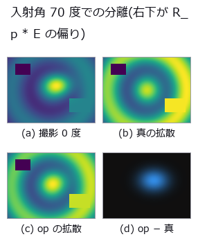
↑ 残差はローブと同じ形。

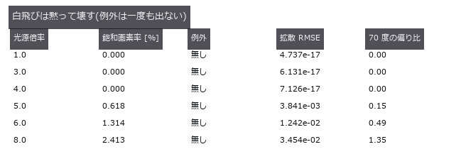
↑ 画素率 1.8 倍で誤差 2.8 倍 —— 雑音(σ に比例)や較正誤差(δ に比例)と違い、飽和は超線形に効く。

py -3.11 examples/poc_polarization_specular.py

Source: examples/poc_polarization_specular.py

This run produced 4 figures in total - see them all

Ops used (notes): fresnel_reflectance · polarization_dolp_map · polarization_render · polarization_separate · polarization_stokes · rmse

No.2026.107 —— Separating a Real Immunostain by Colour — The Watchdog Was Blind to Exactly the Error It Should Catch

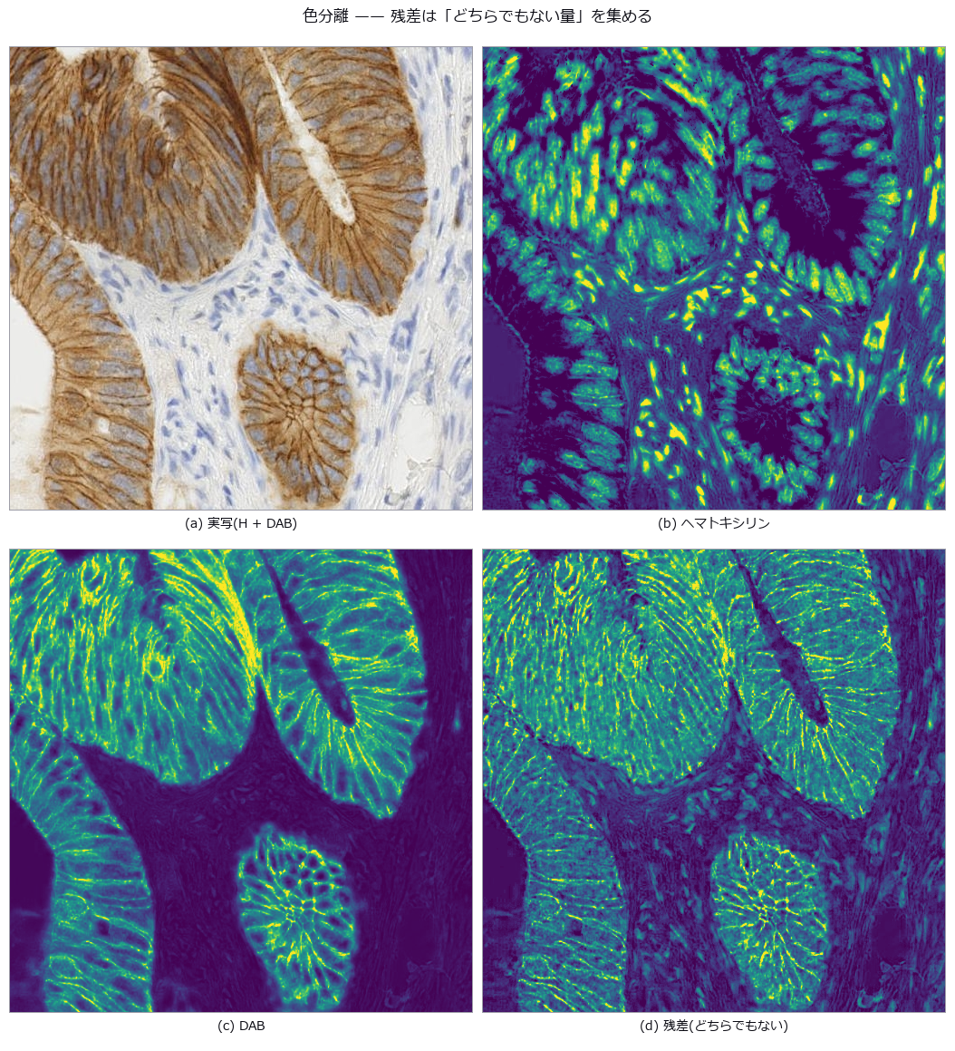
↑ Separating a Real Immunostain by Colour — The Watchdog Was Blind to Exactly the Error It Should Catch ―― Colour deconvolution of a real immunostain (haematoxylin plus DAB). On synthetic data it separates perfectly — recompose one stain at unit concentration, solve again, and recovery is 1.0000 with 0.0000 crosstalk — so anyone looking only at synthesis concludes the problem is solved. On the real slide the haematoxylin concentration runs down to -4.446 and 11.51 % of pixels are negative, which is physically impossible: a negative concentration means the dye emitted light. Rotating the stain vectors within their plane by plus or minus twenty degrees moves the haematoxylin median from 0.0471 to 0.1348, a factor of 2.86, and DAB from 0.3590 to 0.1836 — while the residual channel, the quantity everyone reads as goodness of fit, stays at 0.0345 with a total spread of 3.3e-16. The geometry says why: the plane the two stains span is unchanged by a rotation inside it, so the component orthogonal to that plane cannot move. The negative fraction of the rotated stain is equally blind, fixed at 11.51 %, because its dual vector changes length but not direction. Only the partner moves, from 0.00 % at minus twenty degrees to 30.38 % at plus twenty: the watchdog has to watch the other stain, not itself, and being monotone it bounds the error from one side only. The round trip through recompose closes to 1e-06, which refutes none of this.

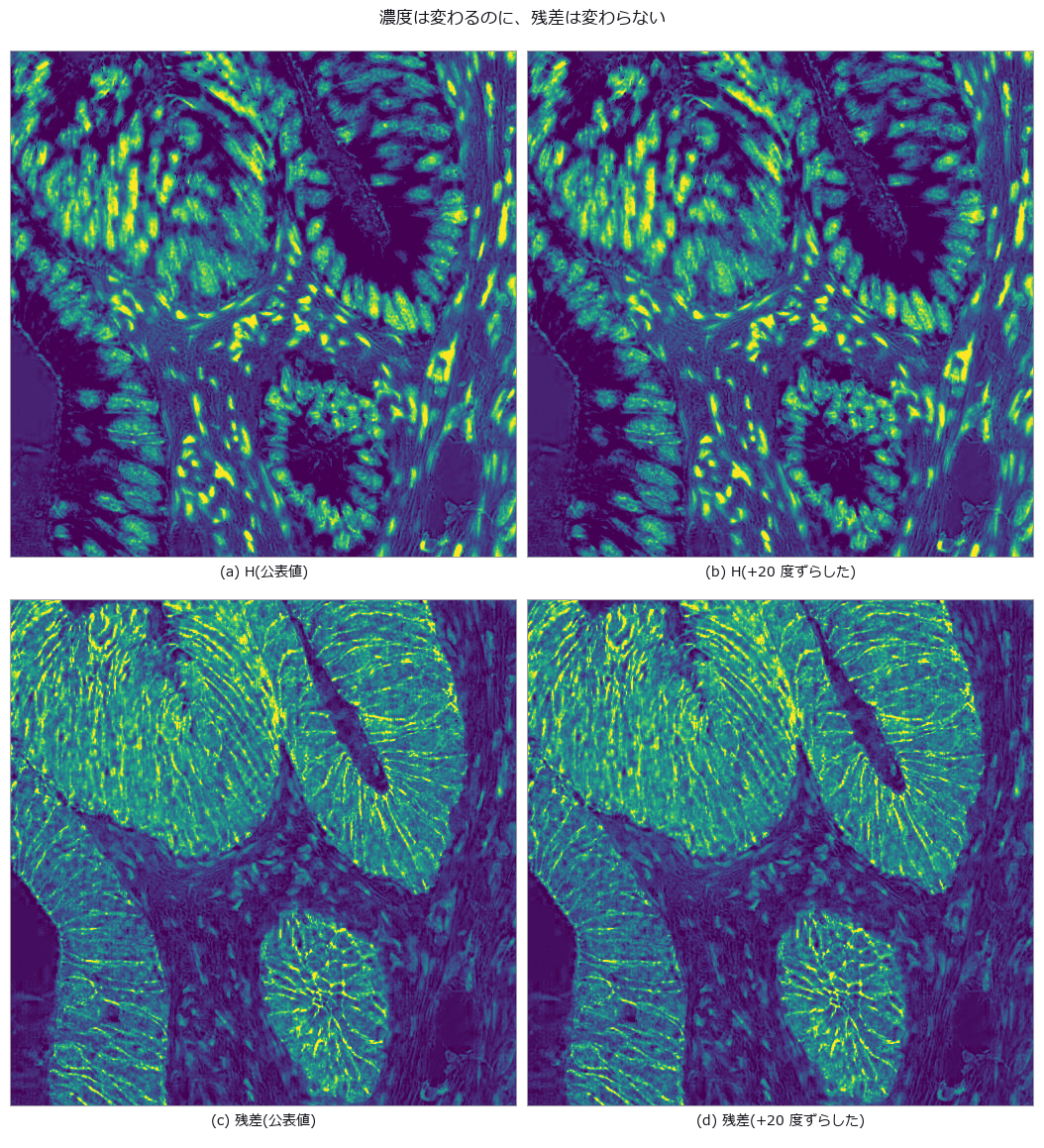
↑ The measurement ―― H の中央値は 0.0656 -> 0.1348。残差の絶対中央値は 0.0345 のまま。 (figure labels are in Japanese; the numbers are the same)

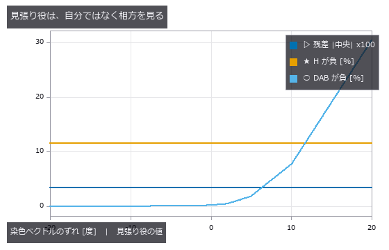
↑ 残差と自分の負率は平坦。

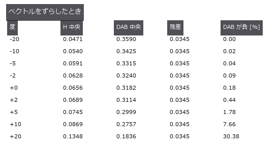
↑ 濃度は 2.9 倍動くのに残差は 4 桁目まで同じ。

py -3.11 examples/poc_real_stain_unmix.py

Source: examples/poc_real_stain_unmix.py

This run produced 4 figures in total - see them all

No.2026.051 —— Colour Constancy (White Balance) — No Method Works, Only Conditions Do

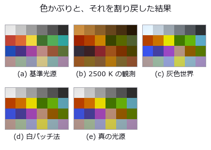
↑ Colour Constancy (White Balance) — No Method Works, Only Conditions Do ―― Linear RGB synthesised from 24 known spectral reflectances and known illuminants, with illuminant estimation scored by recovery angular error. Max-RGB is best at a median of 1.06 degrees over 11 illuminants, but removing the single brightest patch takes it to 8.45 degrees, and tripling exposure to saturate 43 % of pixels takes it to 13.61 degrees, identical to doing nothing. Even a diagonal correction with the true illuminant leaves a mean ΔE00 of 5.07 at 2500 K.

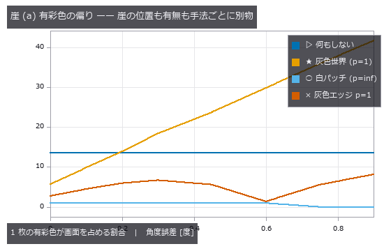
↑ The measurement ―― 灰色世界はゼロ点(何もしない)の線を 0.1〜0.2 の間で上抜けする = そこから先は回すだけ損。白パッチ法には崖が無い。 (figure labels are in Japanese; the numbers are the same)

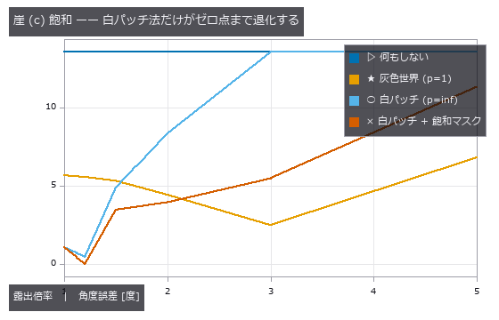
↑ 露出 3 以上で白パッチ法の線が「何もしない」に重なる(max が (1,1,1) に張り付く)。

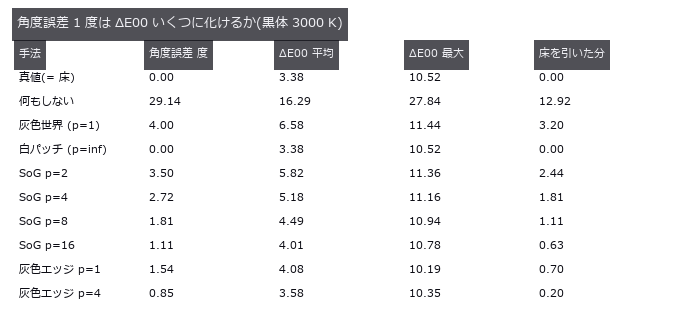
↑ 最右列が推定誤差の実費。

py -3.11 examples/poc_white_balance.py

Source: examples/poc_white_balance.py

This run produced 4 figures in total - see them all

Ops used (notes): delta_e_map · gauss_filter · illuminant_from_dichromatic_planes · laplace · linear_to_srgb · mean_image · prewitt_amp · roberts · sobel_amp · spectrum_to_srgb

The Forensics and Documents Wing — One Successful Image Is Not Evidence

Forgery detection and document rectification. Both tend to be presented through 'the one image where it was found' or 'the one page that came out straight'. The 4 exhibits here fix the paste location and quality, the homography and the lighting themselves, then score with a per-pixel ROC and pixel-level geometric error.

The forgery exhibit is on the detection (defensive) side. Forgeries are generated only because scoring a detector needs ground truth, and the generator is kept to the crudest form possible. What the exhibit shows most strongly is the fact that works against the detector: one press of the save button weakens every cue.

The document exhibit puts a number on a hole: two functions with the same name and different models can be swapped without an exception, returning a plausible picture with the keystone still in it. Shadow removal has no free lunch; the flatter the paper, the more of the faint text disappears.

No.2026.015 —— Straightening a Hand-Held Document Photo — Keystone Correction and Shadow Removal Against Ground Truth

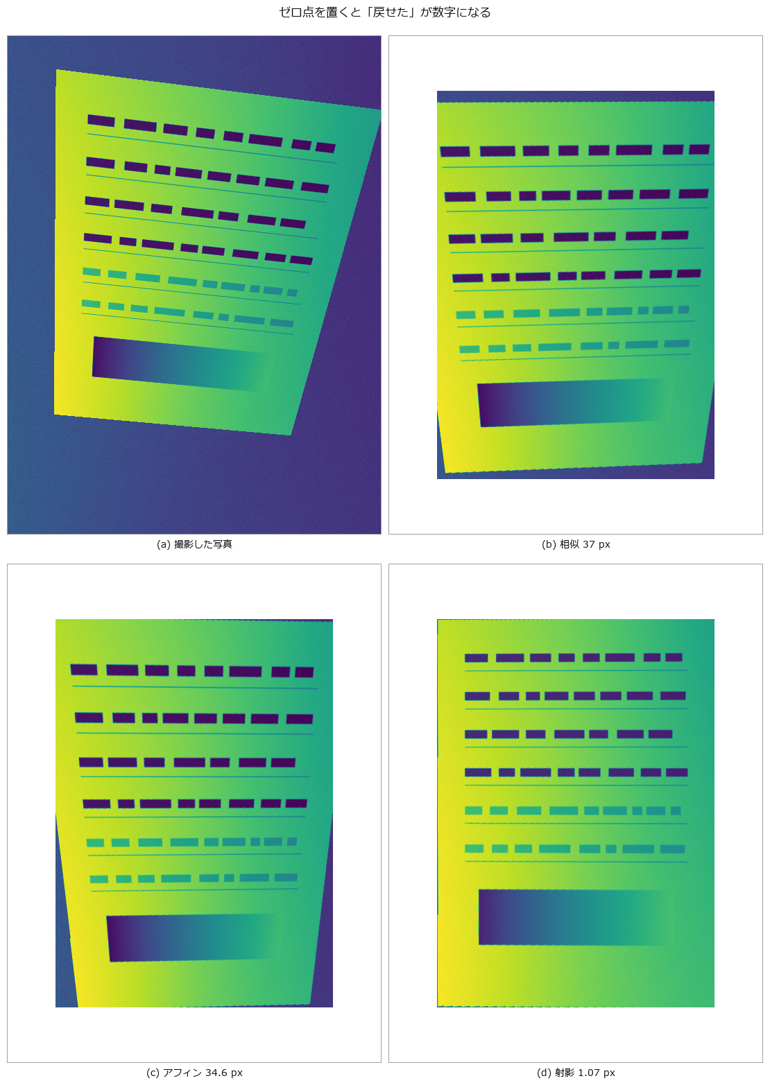
↑ Straightening a Hand-Held Document Photo — Keystone Correction and Shadow Removal Against Ground Truth ―― A document imaged under a known homography and lighting, rectified, and scored by corner and grid error in pixels. The estimate reaches a grid RMS of 1.070 px (doing nothing: 37.376 px), but swapping in the same-named function with a different model (affine) is 32x worse and raises no exception. Shadow strength 0.45 gives a corner RMS of 5.72 px; 0.55 gives 65.10 px — a cliff.

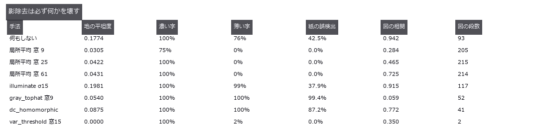
↑ The measurement ―― 平坦・薄字・誤検出なしを同時に満たす行は 1 つも無い。窓 9 が fs.op で届く上限、窓 61 は自前。図の階調は真値で 217 段。 (figure labels are in Japanese; the numbers are the same)

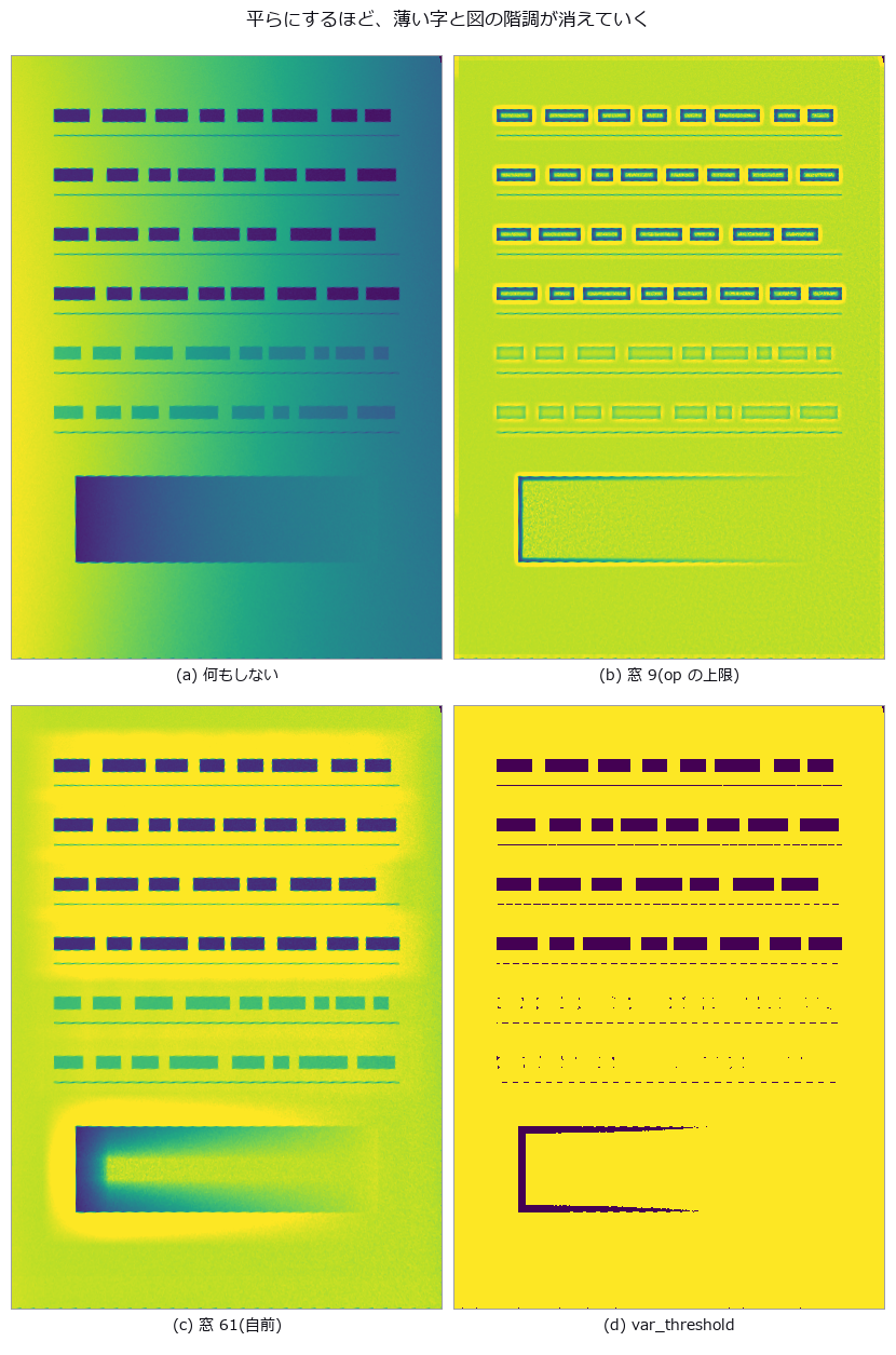
↑ 下寄りの横長の帯が図の階調。

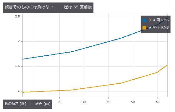
↑ 60 度でも 2 px 台。

py -3.11 examples/poc_document_scan.py

Source: examples/poc_document_scan.py

This run produced 4 figures in total - see them all

Ops used (notes): corner_response · dc_homomorphic · fill_holes · gauss_filter · get_region_contour · gray_tophat · illuminate · mean_image · opening_circle · otsu · project_points · reflect · select_largest · sobel_dir · var_threshold

No.2026.020 —— Forgery Detection as an ROC — Not the One Image Found, but Detection at a Fixed False-Positive Rate

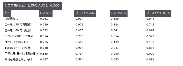
↑ Forgery Detection as an ROC — Not the One Image Found, but Detection at a Fixed False-Positive Rate ―― Ten forgeries made by pasting a JPEG q60 patch onto a q92 background and saving at q95, scored with a per-pixel ROC. ELA's single number points the opposite way from the textbook (paste / background = 0.58x), and an untouched image still yields an AUC of 0.797 from position bias alone. The ghost-valley depth reaches an AUC of 0.997, which falls to 0.975 after one whole-image recompression at q75.

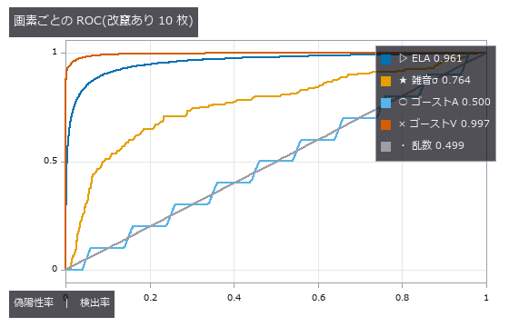
↑ The measurement ―― 凡例の数字は AUC。乱数が対角線に乗ることで測り方に偏りが無いと言える。ゴーストA は乱数と重なる。 (figure labels are in Japanese; the numbers are the same)

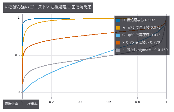
↑ 凡例の数字は AUC。

↑ 保存ボタン 1 回(q60 再圧縮)で ゴーストV は乱数以下。

py -3.11 examples/poc_forensics_roc.py

Source: examples/poc_forensics_roc.py

This run produced 4 figures in total - see them all

Ops used (notes): copy_move_regions · error_level_map · jpeg_ghost_map · jpeg_ghost_quality · noise_inconsistency_map · reflect

No.2026.067 —— Craquelure networks — of three indicators, only junction degree breaks under imaging conditions

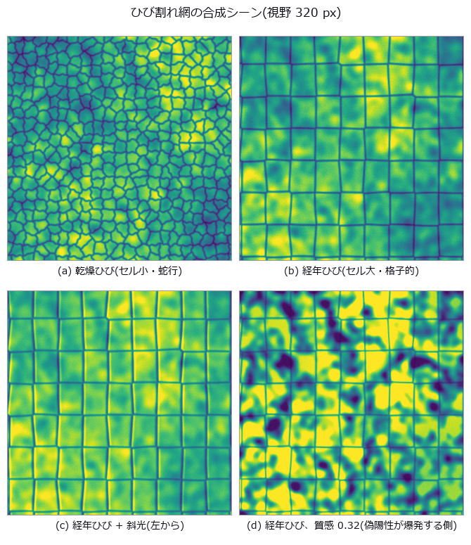
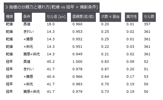
↑ Craquelure networks — of three indicators, only junction degree breaks under imaging conditions ―― A Voronoi crack network is drawn in closed form for two ground-truth types — drying cracks (small tortuous cells) and age cracks (large grid-like cells) — with paint blotches, varnish gloss, raking light, blur and noise, then measured with a ridge op → skeleton → junction chain. Truth separates the types on all three indicators (cell diameter 18.0 vs 45.2 px, straightness 0.960 vs 1.000, degree-4 fraction 0.20 vs 0.83), yet the age type's degree-4 fraction drifts toward the drying value under texture (0.87 → 0.64) and raking light (0.70) while diameter and straightness stay put. Both predicted cliffs failed to appear: recall is still 0.696 at 0.15 px width and false positives only 0.382 at texture contrast 0.64. Raking light widens cracks one-sidedly by +0.37 px and shifts the centreline 0.75 px toward the light.

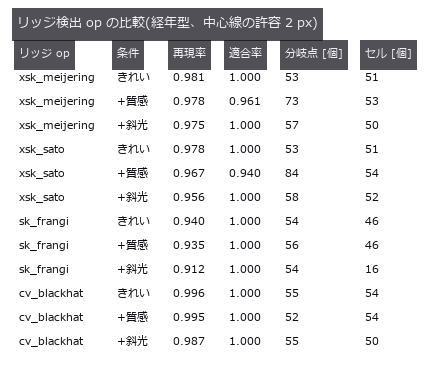
↑ The measurement ―― Frangi は分岐点で応答が落ち、斜光でセルが崩れる。 (figure labels are in Japanese; the numbers are the same)

↑ 真値は幾何(ボロノイの頂点・辺)から。

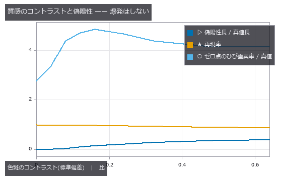
↑ ひびの深さ 0.55。

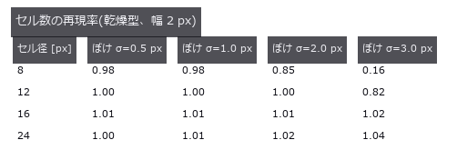
↑ ぼけが大きいほど小さいセルから消える。

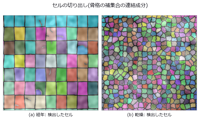
↑ 縁に触れるセルは統計から外す(真値も同じ規約)。

py -3.11 examples/poc_fresco_craquelure.py

Source: examples/poc_fresco_craquelure.py

This run produced 11 figures in total - see them all

Ops used (notes): blob_features · blob_label · blob_overlay · cv_blackhat · distance_transform · hx_split_skeleton_region · hysteresis_threshold · junctions_skeleton · otsu · pruning · r2_endpoints_skeleton · sk_area_opening · sk_frangi · sk_otsu · skeleton · threshold · xsk_meijering · xsk_sato

No.2026.077 —— Camera Fingerprints (PRNU): Which Camera Took This? — The Fingerprint Grows With Frame Count and Dies at the Save Button

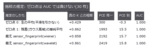
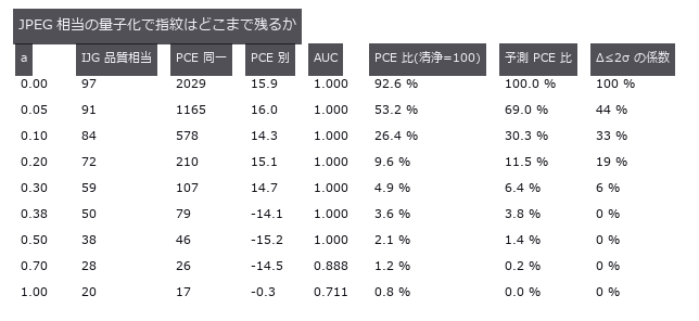
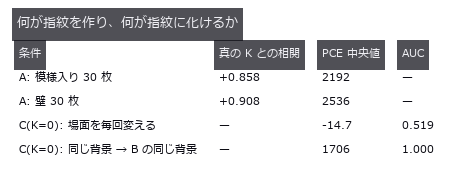
↑ Camera Fingerprints (PRNU): Which Camera Took This? — The Fingerprint Grows With Frame Count and Dies at the Save Button ―― Two virtual cameras carry a fixed sensitivity pattern K; the fingerprint is estimated from 30 residuals and matched. Under clean conditions the same camera scores a median PCE of 2192 against 15.7 for the other (AUC 1.000), but JPEG-like quantisation at quality 50 cuts PCE to 3.6 % and a 0.5x downscale to 1.5 % — and what killed it was the residual extractor, not the geometry. A camera with K = 0 still yields a 'fingerprint' with PCE 1706 if the same background is shot 30 times: the scene turns into a fingerprint.

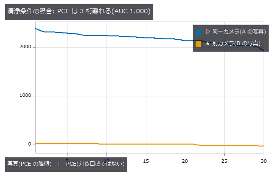
↑ The measurement ―― 別カメラのピークは毎回別の位置に立つ((0,0) は 0/30)。 (figure labels are in Japanese; the numbers are the same)

↑ この回の図

↑ この回の図

↑ 幾何の上限 = K 自身を同じ往復に通した相関²。

↑ この回の図

py -3.11 examples/poc_prnu_camera_fingerprint.py

Source: examples/poc_prnu_camera_fingerprint.py

This run produced 10 figures in total - see them all

Ops used (notes): aug_jpeg_blocks · evidence_quantile · fingerprint_correlate · gauss_image · median_image · null_distribution · reflect · sensor_fingerprint · sk_nlm · sk_tv · sk_wavelet · xsp_dct_denoise · xsp_wiener

The 3-D Shape Wing — Align First, and the Alignment Eats the Defect

Work on point clouds and meshes differs from 2-D work in one decisive way: a pose-alignment step comes before the measurement. That step rotates the shape into whatever orientation makes the discrepancy smallest, so the larger the defect, the more of it the alignment absorbs, leaving a small residual and a part that looks in tolerance. The exhibits in this room try to count what the alignment ate.

Every ground truth here is written as a formula. Solids are built from analytic surfaces combined with boolean operations, chosen so that volume, surface area, wall thickness and curvature are known in closed form. Deformations are known fields (a local dent, a warp, a constant wear along the surface normal), poses are known rotations and translations, and the scan is a uniform sample of the surface with a known density, noise level and occlusion pattern. That is what makes it possible to hold the alignment error and the shape error apart.

The pitfalls specific to 3-D also get counted separately here. A nearest-neighbour distance is biased upward whenever there is noise, because it only ever counts one side. Normal signs are decided by whatever helper computed them. Changing the point density changes the scale of the distance itself. A symmetric shape has no unique pose. Each of these disappears the moment the numbers are folded into one.

No.2026.054 —— Battery cell degradation by CT — the swelling shows outside, the cause stays inside

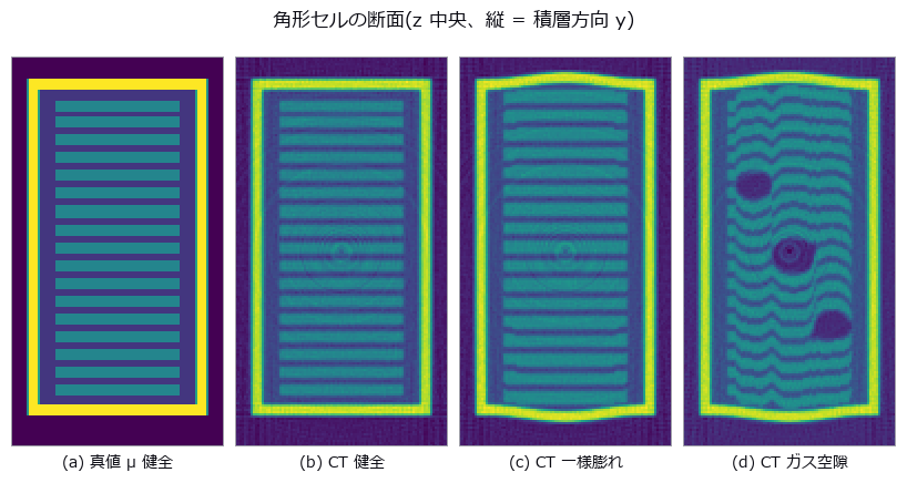
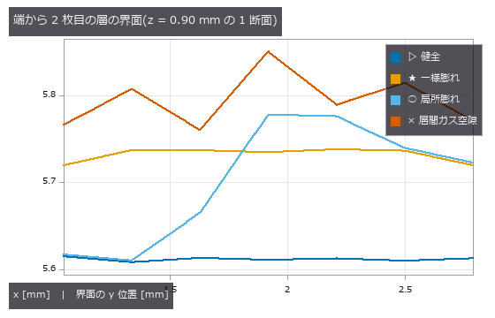
↑ Battery cell degradation by CT — the swelling shows outside, the cause stays inside ―― A prismatic lithium-ion cell — stacked electrodes inside an aluminium can — is built with ground truth, degraded by known fields (uniform swelling, local swelling, inter-layer gas voids, electrode misalignment), and then imaged for real: forward projection, beam hardening, photon noise and FBP reconstruction. Only 29.4 % of a 10 % electrode swelling reaches the outside, and a caliper across the centre reads 3.6 times the volume-equivalent mean (+0.235 vs +0.066 mm). Three cells tuned to the same external bulge differ by 0.000 mm in can height yet separate internally (void fraction 0.00 vs 5.20 %, layer flatness 0.0156 vs 0.0784 mm), and the resolution cliff for those internal numbers is set by the 0.120 mm inter-layer gap, not the 0.200 mm electrode — voxel/thickness = 0.30, where the sampling-theorem prediction said 0.80.

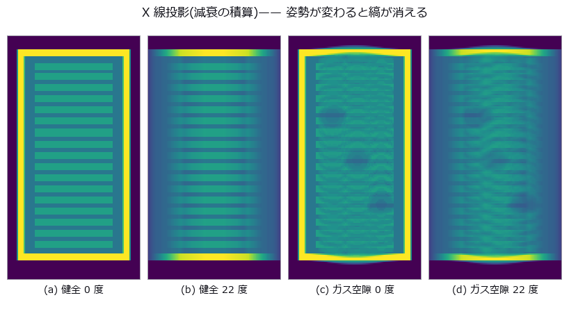
↑ The measurement ―― 真正面(0 度)なら空隙の影までは見える。ただし奥行きに積算されているので厚みも深さも出ない。22 度傾けると層の縞そのものが重なって消える —— 投影では姿勢が結果を決めてしまう。だから断層に落とす。 (figure labels are in Japanese; the numbers are the same)

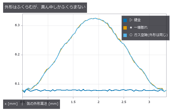
↑ 端板は周辺で固定なので中央だけが出る。

↑ 一様膨れは平らなまま上がる。

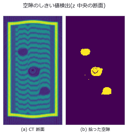
↑ この回の図

↑ 空隙体積は崖の手前から単調に痩せる(部分体積効果)。

py -3.11 examples/poc_battery_ct_degradation.py

Source: examples/poc_battery_ct_degradation.py

This run produced 16 figures in total - see them all

Ops used (notes): beam_hardening_apply · box_sdf · fbp_volume · grid_coords · plane_sdf · projection_angles · radon_volume · render_volume_projection · ring_artifact_apply · sdf_intersect · sdf_subtract · sdf_to_occupancy · sdf_union · vol_bounding_box · vol_edge_probe · vol_fft_lowpass · vol_label · vol_profile_line · vol_region_props · vol_resize · vol_wall_thickness

No.2026.056 —— Fusing two sensors into a bird's-eye grid — a calibration that passes in pixels turns into metres at range

↑ Fusing two sensors into a bird's-eye grid — a calibration that passes in pixels turns into metres at range ―― An analytic street scene (a tall lead truck, plus two distant cars each hidden in the other sensor's shadow) is fused from a left-mirror LiDAR and a right-mirror depth camera into one bird's-eye grid, then swept over rotation, translation and timing errors in the extrinsics. Fusion reaches an occupancy IoU of 0.7033 against 0.5417 for the best single sensor — and every bit of that gain comes from complementary visibility, not accuracy. One pixel of reprojection error becomes 0.083 m at 22 m; the cliff is set by the object width, not the 0.2 m cell (IoU drops only 5.8 % when 68 % of the points have already crossed a cell); by 3 deg of yaw the fusion has fallen below the single sensor.

↑ The measurement ―― 横に 1.80 m 離した 2 センサの「自由と言い切れた領域」。青い帯が LiDAR にしか見えない所、橙の帯がカメラにしか見えない所、灰色は両方。白は真値の障害物。22 m の 2 台は互いの影に 1 台ずつ入っている。 (figure labels are in Japanese; the numbers are the same)

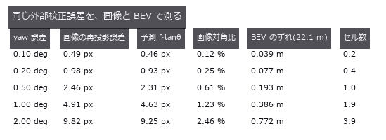
↑ 画像 320 x 240 px、焦点距離 265 px。

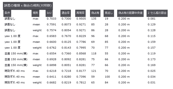
↑ 誤差はカメラ側の外部パラメータにだけ入れる。

↑ LiDAR は 22 m の車を 1 セルも返せない(先行車の陰)。

↑ 水平の 2 本は単センサのゼロ点。

py -3.11 examples/poc_bev_sensor_fusion.py

Source: examples/poc_bev_sensor_fusion.py

This run produced 9 figures in total - see them all

Ops used (notes): box_sdf · closing_circle · depth_to_points · esdf · fill_up · fuse · grid_coords · occupancy_grid · project_points · sdf_to_occupancy · sdf_union · voxel_grid_downsample · voxel_iou

No.2026.058 —— CAD-to-scan deviation inspection — the fit absorbs the defect and invents a dent

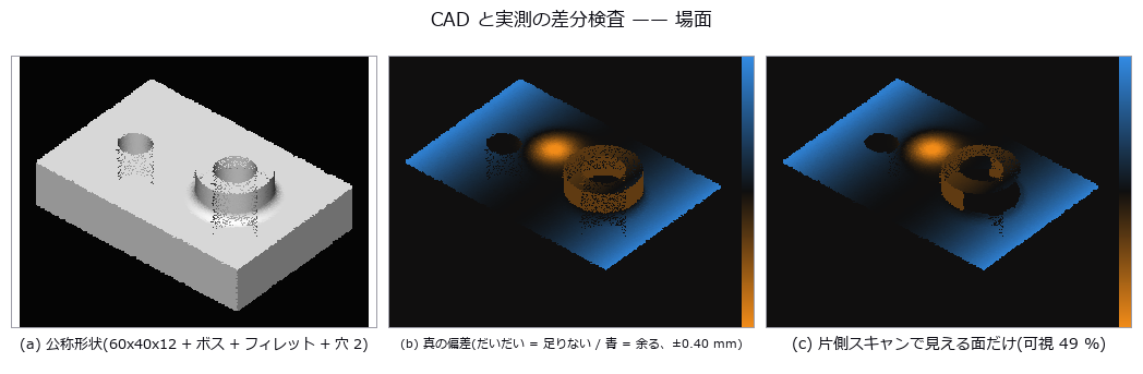
↑ CAD-to-scan deviation inspection — the fit absorbs the defect and invents a dent ―― An analytic machined part carries a known local dent, a bow and a wear band, all applied as exact displacements along the surface normal, and the scan is synthesized with a known pose, noise and one-sided occlusion. After alignment the signed deviation and the out-of-tolerance area show that the local dent is diluted by only 3.7 %, while a 121 um dent appears at the centre of the part where the truth is just 1.2 um (closed form predicts -120 um). What survives depends on how much the defect resembles the six rigid-body degrees of freedom; along the edges the nearest neighbour jumps to the adjacent face, producing 66.5 mm^2 of false out-of-tolerance area even in a defect-free control.

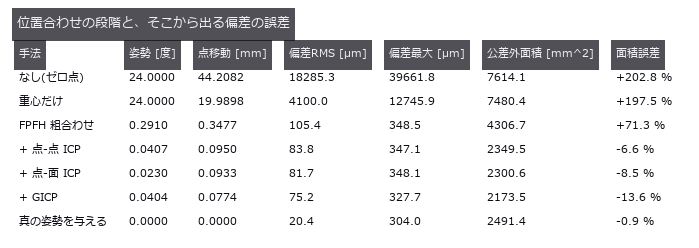
↑ The measurement ―― 真の姿勢を与えた最終行が推定器そのものの床。点-面 ICP との差は姿勢ではなく datum の取り方の差。 (figure labels are in Japanese; the numbers are the same)

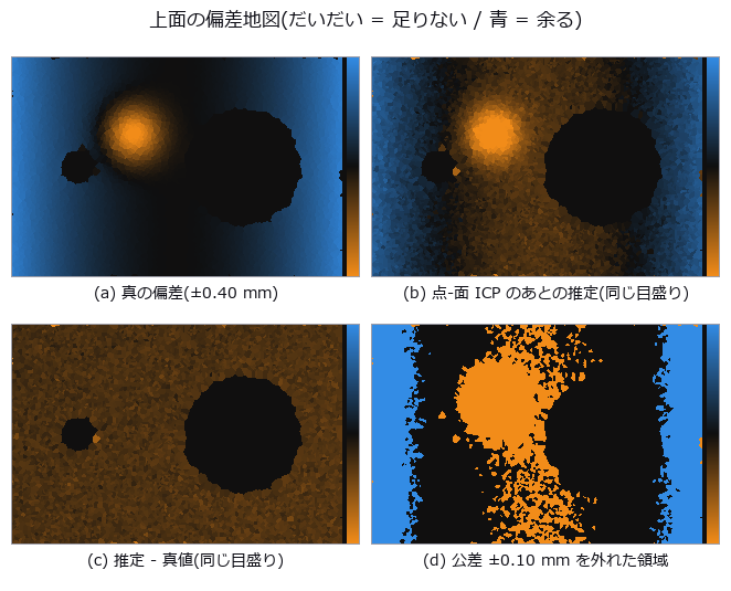
↑ 3 枚目が一様に色づくのが第 6 章の主張 —— 位置合わせが反りの平均を吸って、部品全体が下へずれて読める。

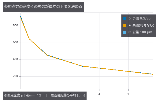
↑ 2 次元 Poisson 点過程の最近傍距離の平均 = 0.5/√ρ。

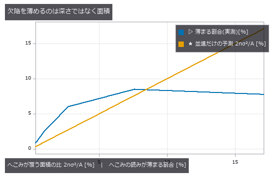
↑ 深さを 30 倍にしても割合は動かないが、広がりを変えると比例して増える。

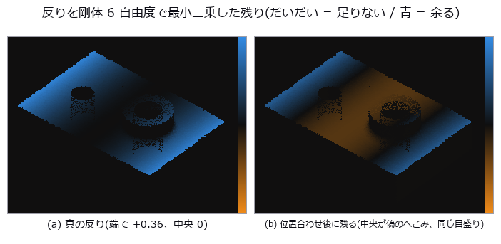
↑ 上面だけを見ている。

py -3.11 examples/poc_cad_scan_deviation.py

Source: examples/poc_cad_scan_deviation.py

This run produced 13 figures in total - see them all

Ops used (notes): box_sdf · chamfer_distance · esdf · estimate_normals · estimate_oriented_normals · face_areas · gicp · hausdorff_distance · icp_point2plane · icp_point2point_3d · query_distance · register_fpfh · sphere_sdf · voxel_grid_downsample

No.2026.063 —— Crop leaf area from above — folded by projection before it is ever hidden

↑ Crop leaf area from above — folded by projection before it is ever hidden ―― A maize canopy built from analytic leaf surfaces (one-sided area pi/4·L·W, leaf angle and projection coefficient both closed-form) is viewed through an exact nadir z-buffer to measure cover, occlusion and leaf angle. Inverting cover with Beer-Lambert underestimates a true leaf area index of 4.85 by 52.2 % even with the exact extinction coefficient, and stalls just above the ceiling of 2.26 predicted from two-scale clumping (measured 2.70). Occlusion changes nadir cover by not one bit; what breaks the estimate is the folding of projection — an average of 3.49 leaves cover a cell yet are counted once — and quadrupling point density buys only +1.92 in the largest resolvable index.

↑ The measurement ―― 閉形式 2 pi r h + 4 pi r^2 / pi r^2 h + 4/3 pi r^3 と比べる。2 値化を挟むと面積だけが一方向に膨らむ。 (figure labels are in Japanese; the numbers are the same)

↑ 稈カプセルの符号付き距離場(縦断面、中心が内側 = 負)

↑ 重なりの枚数(遮蔽を無視して全部数えた場合)は真値に乗る。

↑ この回の図

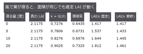
↑ この回の図

py -3.11 examples/poc_crop_phenotyping.py

Source: examples/poc_crop_phenotyping.py

This run produced 17 figures in total - see them all

Ops used (notes): boundary_vertices · capsule_sdf · dem_slope · estimate_normals · face_areas · face_normals · grid_coords · mesh_area · mesh_sample_points · mesh_volume · occupancy_grid · plane_segmentation · render_volume_projection · sdf_to_occupancy

No.2026.064 —— Collapsing joint voids into one number — what the number drops is the shape that matters

↑ Collapsing joint voids into one number — what the number drops is the shape that matters ―― A synthetic die-attach bond line carries five void populations whose volume fraction is held exactly at 3.000 % while only their depth, shape and proximity change, re-imaged as an X-ray CT with a PSF, noise and beam-hardening cupping. The naive zero point — threshold, then report void fraction — separates the five conditions by only 0.17 points (2.46 to 2.63 %), yet the interface area shadowed by flat voids is 2.09x that of volume-matched spheres (14.49 vs 6.92 %) and the largest cluster spans 13.1x further when the voids are chained (80.0 vs 6.1 %). The predicted cliff never arrives: at 60 um voxels the void fraction still reads 3.21 % (it only wobbles by 1.36 points with the grid phase), while flatness becomes unmeasurable and the interface-deficit metric drops from 14.16 to 9.78 % — the degradation runs toward 'pass', which is the worst possible direction.

↑ The measurement ―― 疑似カラーはラベル番号を並べ替えたもの。側面図で界面(上端)に貼りついているのが見える。 (figure labels are in Japanese; the numbers are the same)

↑ ボイド率の列だけを見ると 5 条件は区別できない。

↑ 界面欠損率は 球/中央/散 0.0 % / 球/界面/散 6.9 % / 扁平/界面/散 14.5 % / 球/中央/連 0.0 % / 扁平/界面/連 14.7 % —— 体積率が同じでも 0 から 14.7 % まで動く。

↑ 60 µm では扁平度が測れない(nan なので描けない)。

↑ 塊の数が 24 から落ちた瞬間、最近接間隔は『隣のボイドまで』から『隣の鎖まで』に黙って入れ替わる。

py -3.11 examples/poc_ct_void_morphology.py

Source: examples/poc_ct_void_morphology.py

This run produced 12 figures in total - see them all

Ops used (notes): boundary_vertices · box_sdf · cylinder_sdf · esdf · face_areas · mesh_volume · morph_dilate3d · plane_sdf · query_distance · sdf_union · sphere_sdf · vol_boundary_points · vol_gaussian_psf · voxel_to_mips

No.2026.065 —— Manufacturability from geometry alone — faces that sit on the threshold flip when you smooth them

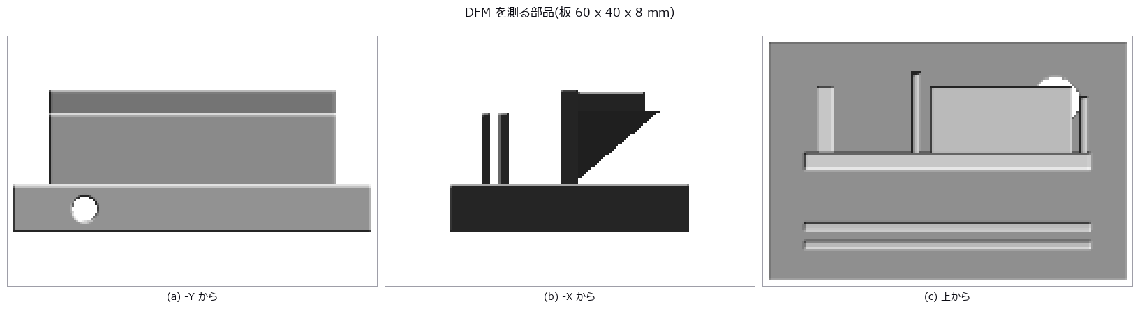
↑ Manufacturability from geometry alone — faces that sit on the threshold flip when you smooth them ―― A synthetic part with known design values (thin walls, a slot, ribs near 45 deg, holes) is voxelised, then wall thickness, support area and tool clearance are measured. Across the 45 deg threshold the support area jumps 185.22 -> 576.10 mm^2 — 3.11x for 0.2 deg — and that step vanishes entirely when the isosurface is taken from a distance field, and loses 12 % under smoothing. Thickness collapses onto a 2-voxel lattice (the inscribed sphere does not help), and clearance errors go both ways: at 0.500 mm voxels the slot appears 2.000 mm wide and admits a tool that does not fit.

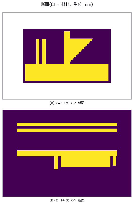
↑ The measurement ―― 上: 左端の 2 本が薄壁(1.500 mm)とそのあいだのスロット(1.500 mm)、右の三角が補強。下: リブと薄壁の footprint。 (figure labels are in Japanese; the numbers are the same)

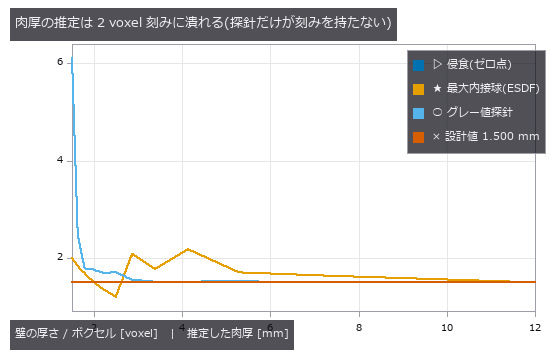
↑ 右ほど粗い。

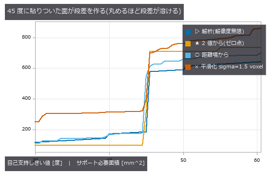
↑ 解析は階段。

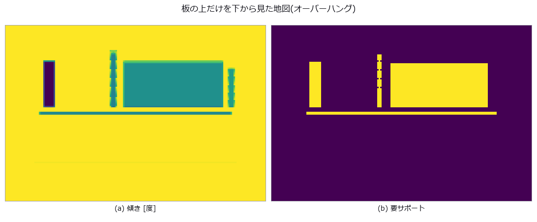
↑ 左 = 水平からの傾き(暗い = 0 度 = 最悪、明るい = 90 度 = 垂直)。

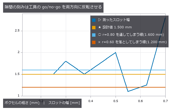
↑ 1.600 mm を超えると入らない工具を通し、1.200 mm を切ると入る工具を落とす。

py -3.11 examples/poc_dfm_thickness_overhang.py

Source: examples/poc_dfm_thickness_overhang.py

This run produced 9 figures in total - see them all

Ops used (notes): box_sdf · esdf · face_areas · face_normals · grid_coords · morph_erode3d · render_shaded · sdf_intersect · sdf_subtract · sdf_to_occupancy · sdf_union · vol_wall_thickness · voxel_to_mesh

No.2026.070 —— Earthwork on a slope — align first and the scar gets shallower

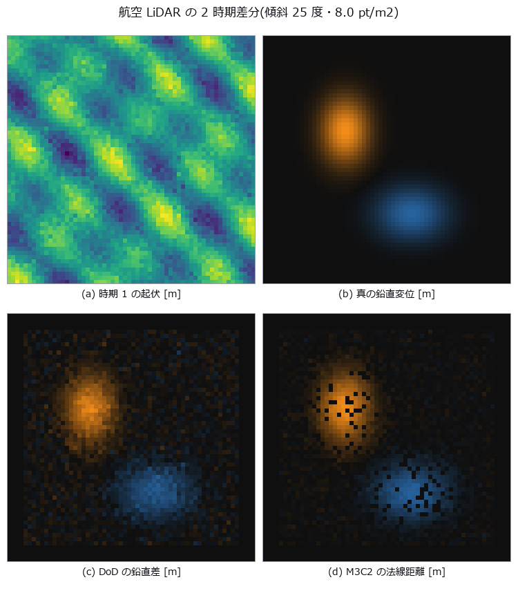
↑ Earthwork on a slope — align first and the scar gets shallower ―― A synthetic slope carries an excavation and a deposit of known volume; two epochs of airborne points are differenced both vertically (DoD) and along the local surface normal (M3C2). The expected "cos-θ shrinkage on a slope" never appears — integrating vertical differences over horizontal area cancels the cosine, and the excavated volume stays within -0.011 % from 0 to 40 degrees. What breaks is the registration: when the changed area covers 33 % of the scene, ICP absorbs the change itself and the net volume collapses from a true -30.4 m3 to -3.8 m3, while a no-change control alone already fabricates 83.8 m3 of phantom excavation.

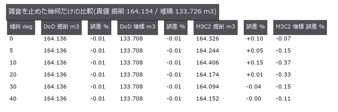
↑ The measurement ―― 傾斜を 0 から 40 度まで振っても体積の誤差に傾向が無い。cos は積分で約分する。 (figure labels are in Japanese; the numbers are the same)

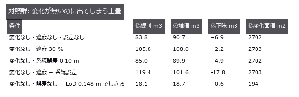
↑ 真の掘削は 164.2 m3。

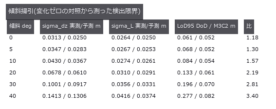
↑ 予測式は先に立ててから測った。

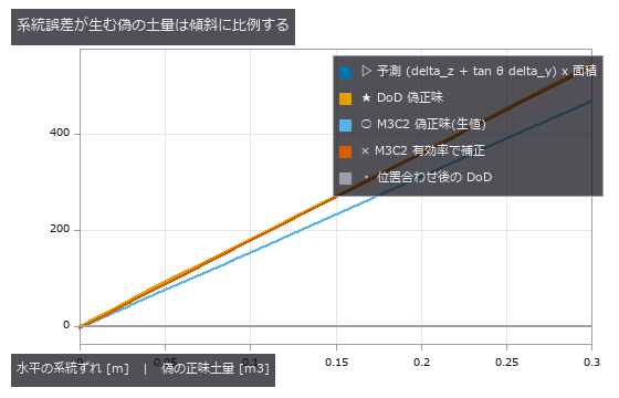
↑ 変化ゼロの対照。

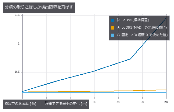
↑ 取りこぼしは 1 % 未満でも、樹冠は数 m 高いので標準偏差だけが桁で跳ねる。

py -3.11 examples/poc_lidar_terrain_change.py

Source: examples/poc_lidar_terrain_change.py

This run produced 11 figures in total - see them all

Ops used (notes): chamfer_distance · estimate_normals · estimate_oriented_normals · fit_plane_3d · icp_point2point_3d · median · ransac_plane · voxel_grid_downsample

No.2026.099 —— Weighing an Animal from Silhouettes — The Error You Can Buy Down, and the One You Cannot

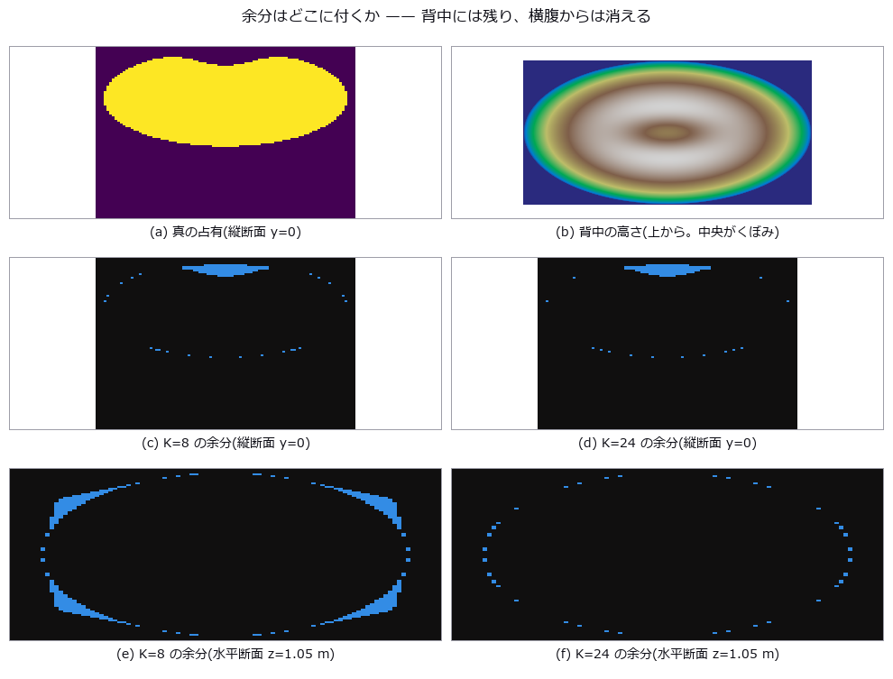
↑ Weighing an Animal from Silhouettes — The Error You Can Buy Down, and the One You Cannot ―― Estimate an animal's volume from the intersection of multi-view silhouettes (the visual hull) and convert it to weight. A visual hull is always an upper bound, so the question is not whether it is good but that it is always high. The closed form corrected the field rule of thumb: K cameras do not give a K-gon. Under parallel projection each camera contributes two support lines perpendicular to its line of sight, and two opposing cameras contribute the same pair, so the number of distinct tangents is K for even K and 2K for odd K. Three cameras and six cameras are therefore geometrically identical (closed form 1.16772 both times, the measured 0.013 difference being discretisation only), half of an even rig is wasted, and 13 cameras (1.03056) beat 16 (1.04768). Requiring 2 % on weight needs 13 cameras if odd counts are allowed and 24 if not — the naive circular reading of (K/pi)tan(pi/K) says 13, so a team building an even-numbered rig is short by 11. Against the exact ellipse (a/b = 2.76) the measurements sit just above the closed form at every K, confirming it as a lower bound. The centre of this exhibit is separating the error you can buy down from the one you cannot: the phantom between the legs falls from 7.13 % to 1.37 % going from 4 to 48 cameras, while the hollow of the back falls only 3.8 points (56.4 % to 52.6 %) for the same twelvefold increase, because a concavity that never reaches the outline leaves no trace in any silhouette. One pixel of segmentation error is likewise unbuyable, worth +3.21 % per pixel (23.7 kg), matching Steiner's dV/V = (S/V)delta to a ratio of 1.04 — though the text records that two opposing effects happened to cancel there. The rulers disagree on the winner: volume-derived and allometric weight both prefer 24 cameras with a two-pixel erosion, while the height of the centroid prefers no erosion at all, since the thin legs disappear first. One prediction was wrong: a tape measure wraps the body, so the 3-D convex hull was expected to be the strong method for heart girth, but it measured +55.2 % — the hull of the whole body fills in under the belly and drags the cross-section down to the ground. The convex hull of a section and the section of a convex hull are not the same object. A tooling hole was found and closed on the way: the OpenCV-convention pose helper that space carving requires was unreachable from every public tier, while the name look_at in the public API belonged to the OpenGL-convention version, so grabbing the wrong one returned an empty hull with no exception at all.

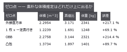
↑ The measurement ―― 真値 0.7238 m^3 / 738 kg。外接直方体と OBB は上界の中でもいちばん粗い。 (figure labels are in Japanese; the numbers are the same)

↑ 法線は方位 ± 90 度。

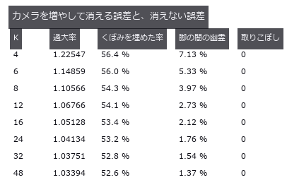
↑ くぼみ(輪郭に出ない凹み)は台数に鈍感、脚の間(輪郭に出る凹み)は台数に敏感。

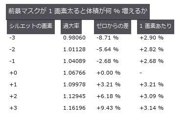
↑ K=12・4.0 mm/px。

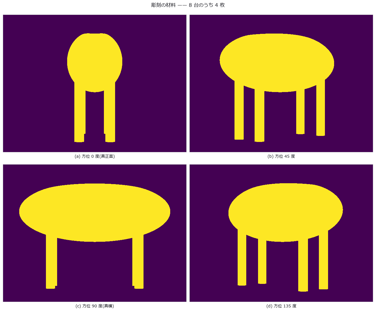
↑ 脚の間の空隙はどの 1 枚にも写っている(だから彫れる)。

py -3.11 examples/poc_livestock_body_volume.py

Source: examples/poc_livestock_body_volume.py

This run produced 13 figures in total - see them all

Ops used (notes): carve · carve_look_at · convex_hull · erosion_circle · mesh_volume · synthesize_silhouette · vol_rle_bbox · vol_rle_centroid · vol_rle_encode · vol_rle_volume

No.2026.072 —— Repair the mesh, then measure — the defect count clears, the quantity does not

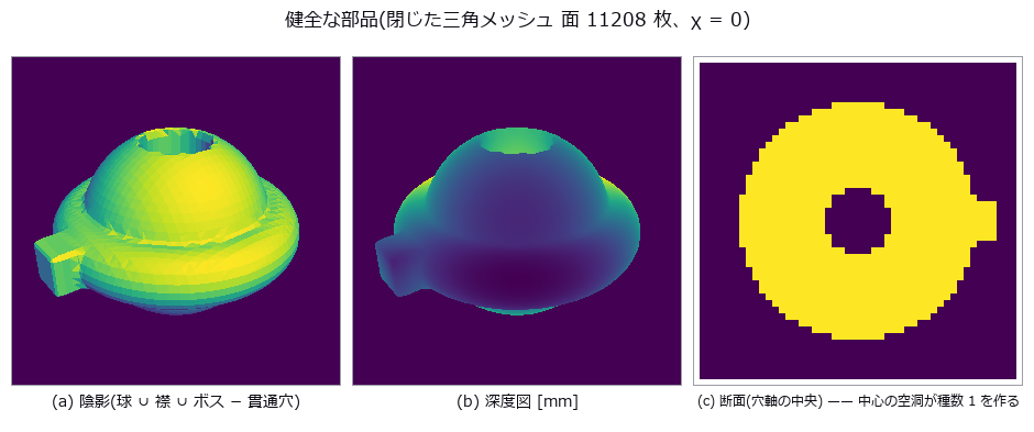
↑ Repair the mesh, then measure — the defect count clears, the quantity does not ―― A closed triangle mesh is built from the boolean union of a sphere, a torus and a box, then seeded with a known count of each defect class — holes, flipped faces, non-manifold edges, degenerate slivers, duplicated vertices and self-intersection — and tracked with both the topological counts and the volume/area. The Euler characteristic does not move at all for 5 of the 6 classes, and 6 holes plus 6 duplicated faces leave the vertex, edge, face and chi counts identical to the healthy part. Repair does not bring the quantities back: filling a 45-degree cap hole on a sphere changes the surface area by +6.868 % where the closed form predicts -2.145 % (the rim is a staircase, not a circle), and pushing just 6 vertices inward passes all three topological checks while the area is +4.414 % and the volume -0.332 % — a 13-fold disagreement.

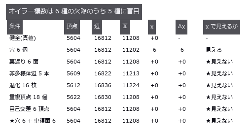
↑ The measurement ―― 健全な部品の χ は 0(種数 1)。χ=2 を合格条件にすると健全品が落ちる。最終行は打ち消し。 (figure labels are in Japanese; the numbers are the same)

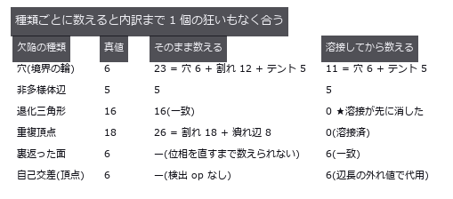
↑ ただし順番が両向きに効く —— 溶接前は割れの境界を穴として数え、溶接後は退化三角形を数え損ねる。

↑ 幅ゼロの割れ(重複頂点 18 個)を直した結果。

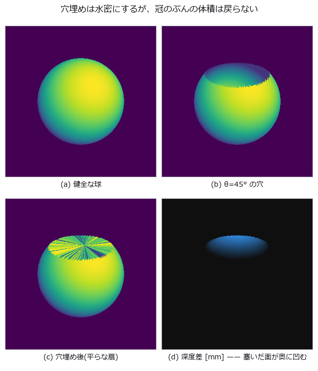
↑ この回の図

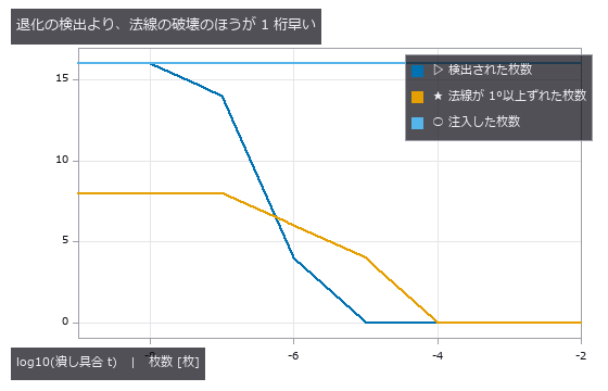
↑ 面積 0 の判定に引っかかるずっと手前で、潰れ面の法線は使いものにならなくなる。

py -3.11 examples/poc_mesh_quality_repair.py

Source: examples/poc_mesh_quality_repair.py

This run produced 13 figures in total - see them all

Ops used (notes): decimate_qem · face_normals · fill_holes · inertia_tensor · mesh_area · mesh_edge_lengths · mesh_edge_stats · sdf_subtract · sdf_union · vertex_curvature · vertex_normals · voxel_to_mesh

No.2026.101 —— Pallet load utilization — one number gives voids and overhang the same value

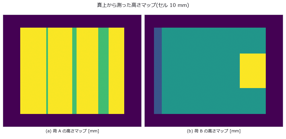
↑ Pallet load utilization — one number gives voids and overhang the same value ―― Two loads with opposite defects sit on a 1200 x 1000 mm pallet: load A hides a 400 x 400 x 420 mm cavity under a bridging layer plus 20 / 50 / 120 mm slots, while load B is solid but overhangs by 90 mm and tops out 100 mm above the 1800 mm limit. Solving the middle-layer height in closed form (995.0 mm) makes their apparent utilization identical — 62.65 % vs 62.67 %, a 0.02 pt gap — yet A's 3.11 pt is invisible void and B's is 2.10 pt overhang plus 0.58 pt over-height, so one load gets restacked and the other gets rejected. Treating the load as one envelope reports 113.90 % (AABB) and 166.44 % (PCA box) for load B, and the IoU between the true solid and the top-down extrusion is 0.9493 / 1.0000 — both read as 'good agreement'. One knob, the height-map cell size, breaks the answer in two opposite directions: a slot of width w survives only as max(0, 1 - g/w) (a 20 mm slot is gone at g = 40 mm, and at g = w exactly the grid phase decides all-or-nothing — 1 alignment in 5 sees everything), while a load that overhangs by nothing acquires a false overhang of perimeter x g/2 x height that overtakes load B's genuine 0.0450 m3 from g = 40 mm on.

↑ The measurement (figure labels are in Japanese; the numbers are the same)

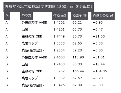
↑ この回の図

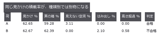
↑ この回の図

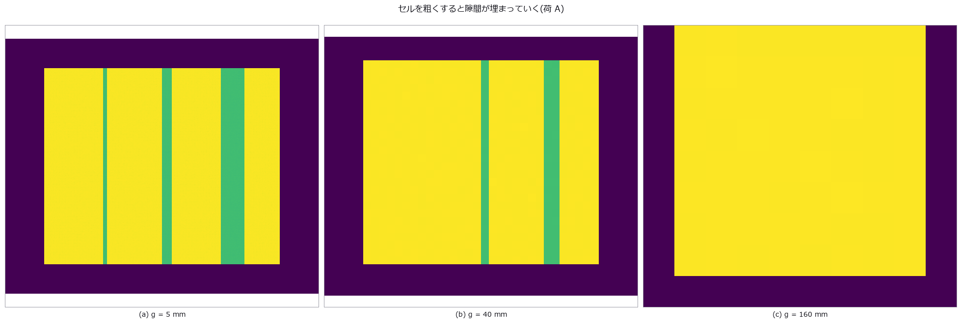
↑ この回の図

↑ この回の図

py -3.11 examples/poc_pallet_load_utilization.py

Source: examples/poc_pallet_load_utilization.py

This run produced 8 figures in total - see them all

Ops used (notes): aabb · convex_hull · euclidean_cluster · inner_box3 · mesh_volume · voxel_iou

No.2026.075 —— Pipe Wall Loss on the Unwrapped Map — The Axis You Choose Eats the Invert Corrosion

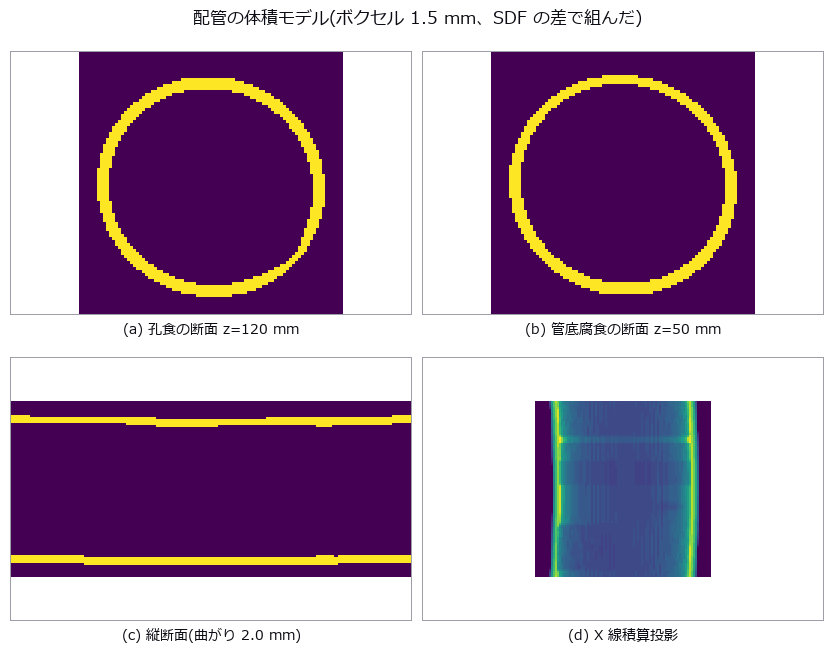
↑ Pipe Wall Loss on the Unwrapped Map — The Axis You Choose Eats the Invert Corrosion ―― A synthetic pipe carries a pit, a full-circumference thinning band, invert corrosion, a weld bead, ovality and a sagging axis, all at known depths; the in-pipe range sensor is then deliberately run off-axis before the bore is unwrapped. A 4.0 mm axis offset alone flags 44.8 % of a corrosion-free round pipe as wall loss — within 1.84 points of the geometric prediction that an offset e appears as a one-cycle sinusoid of amplitude e — and the fictitious loss volume is 149.9 times the real pit. Removing the one-cycle term removes the fiction, but 79 % of invert corrosion (the commonest defect in sewers) lives in that same harmonic, so its detection falls from 100.0 % to 34.4 %; only constraining the axis the way physics does (a straight line plus a sag) keeps both.

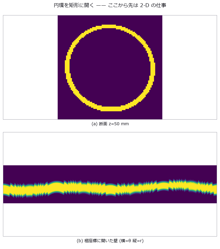
↑ The measurement ―― 下の帯の細くなっている所が管底腐食。 (figure labels are in Japanese; the numbers are the same)

[

↑ 真の減肉 [mm](縦 = z 0..300 mm、横 = θ 0..360 度。

↑ この回の図

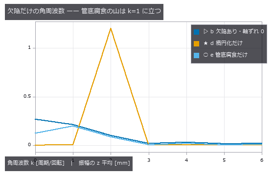
↑ 楕円化は k=2 に立つので分離できる。

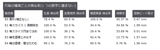
↑ この回の図

py -3.11 examples/poc_pipe_wall_loss.py

Source: examples/poc_pipe_wall_loss.py

This run produced 19 figures in total - see them all

Ops used (notes): blob_label · blob_select · cylinder_sdf · esdf · polar_unwrap · ransac_cylinder · render_volume_projection · sdf_subtract · sdf_to_occupancy · spectrum · vol_wall_thickness

No.2026.076 —— Warpage lives in the layer history — averaging the area throws the placement away

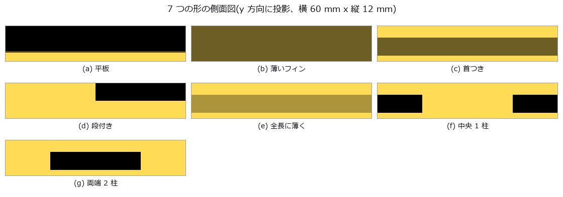
↑ Warpage lives in the layer history — averaging the area throws the placement away ―― Seven synthetic parts are sliced into layers with a known constant per-layer shrinkage strain; warpage is first predicted in closed form from the layer-area history alone, then measured with an incremental layer-birth finite-element solve. A predictor that looks only at the final shape returns exactly zero (2.712e-21), and the history-based closed form lands within 0.4 % on 4 of the 7 shapes — but the moment the area is averaged along the length, where the material sits is lost. Three parts whose layer-area histories match to the last square millimetre bow by 0.4109 / 0.3809 / 0.3271 mm (a 26 % spread), and the force peeling them off the build plate differs by 48x (11.8 vs 573.5 N), flipping the pass/fail verdict.

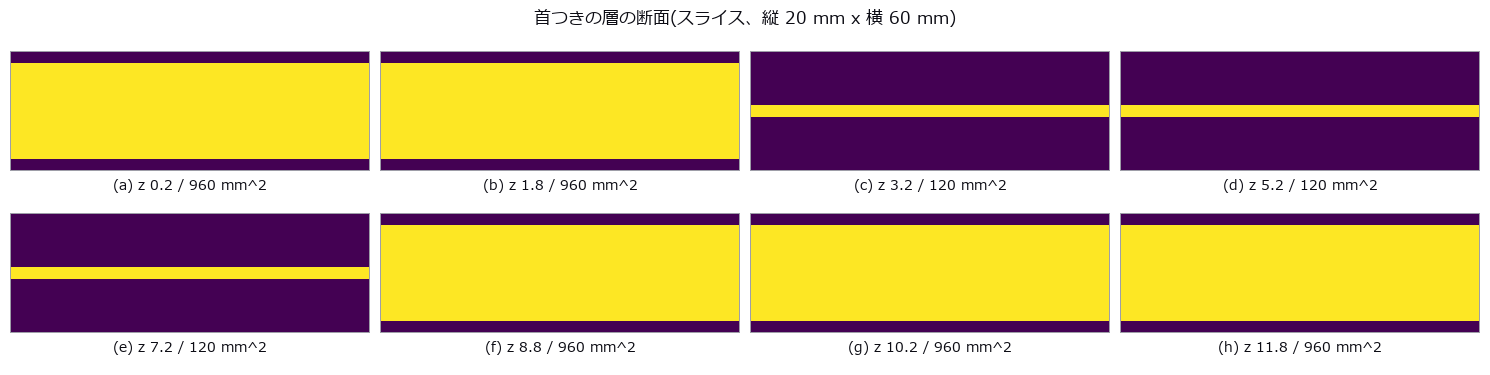
↑ The measurement ―― この断面の面積の列だけが、閉形式の入力になる。 (figure labels are in Japanese; the numbers are the same)

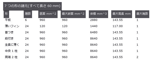
↑ この回の図

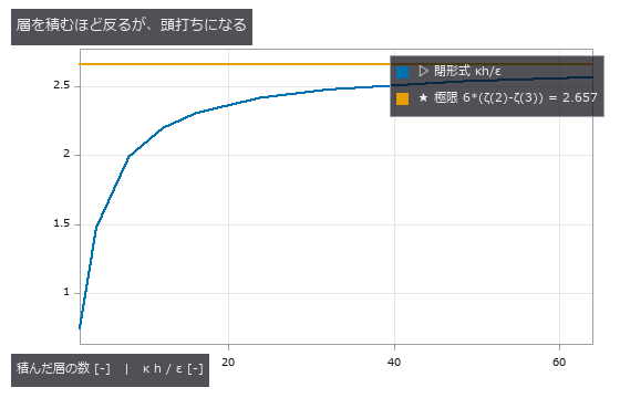
↑ 断面 2 次モーメントが層数の 3 乗で増えるのに、腕は 1 乗でしか伸びないため。

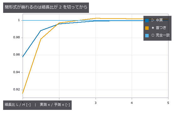
↑ 首の細さでは崩れない(別図)。

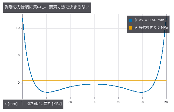
↑ 正 = 接着剤が引っ張られる。

py -3.11 examples/poc_print_warpage_risk.py

Source: examples/poc_print_warpage_risk.py

This run produced 20 figures in total - see them all

Ops used (notes): blob_features · blob_label · box_sdf · grid_coords · render_volume_projection · sdf_to_occupancy · sdf_union · text_box

No.2026.081 —— Human-machine clearance — swap the body for a point, and the hazard vanishes with it

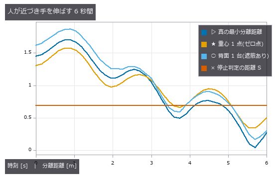
↑ Human-machine clearance — swap the body for a point, and the hazard vanishes with it ―― A ten-capsule articulated body and a moving arm are synthesised so that the true surface-to-surface minimum separation is known in closed form at every instant, and the speed-and-separation-monitoring verdict is then scored against it. Representing the person by one centroid inside a 0.30 m sphere reports the distance +0.166 m too far while a hazard is present and misses 14.3 % of the dangerous frames (28.6 % for a foot-level scanner) — with almost no false alarms, so the failure is strictly one-sided. With a single camera behind the person, 48.6 % of the dangerous frames have the estimate decided by a body part that is not the true nearest one, and 18.1 % are missed; a second camera restores 0 %, but the uncertainty claimed from repeatability, 0.036 m, is only one fifth of the 0.178 m bias that occlusion actually produces.

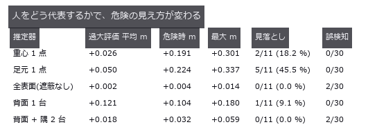
↑ The measurement ―― 危険 = 真の距離 < 0.640 m、停止判定 = 推定 < 0.690 m。 (figure labels are in Japanese; the numbers are the same)

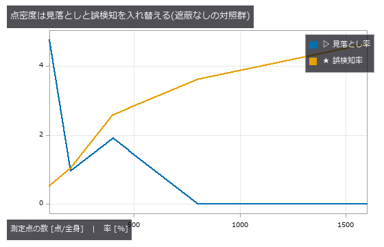
↑ 疎にするほど推定は遠くなるので、誤検知が減って見落としが増える。

[

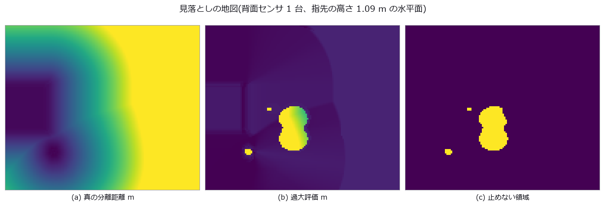
↑ 横 = x [-0.2, 2.2] m、縦 = y [-1.1, 1.1] m。

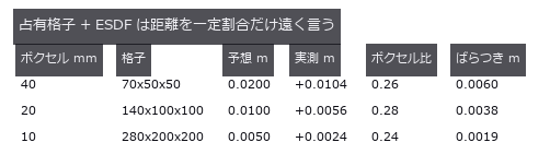
↑ この回の図

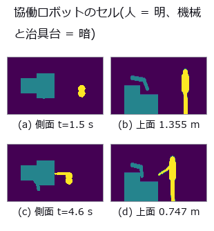
↑ 人は 10 本のカプセル、機械は 2 本のリンク + 基台、手前は治具台。

py -3.11 examples/poc_safety_clearance.py

Source: examples/poc_safety_clearance.py

This run produced 14 figures in total - see them all

Ops used (notes): annotate3d_label · annotate3d_measure · box_sdf · capsule_sdf · chamfer_distance · distance_line_line · esdf · face_areas · hausdorff_distance · query_distance · render_volume_projection · sdf_to_occupancy · sdf_union

No.2026.082 —— As-built deviation of a room — the compromise pose is handed to the innocent element

↑ As-built deviation of a room — the compromise pose is handed to the innocent element ―― A synthetic room carries known construction errors — leaning walls, a sloping and sagging floor, off-size columns, displaced openings — and is re-measured by a simulated scan from three stations with column shadows, incidence-dependent noise, mixed pixels and registration error. One number for the whole building (mean distance to the design model) moves by only 1.41 mm between a perfect building and a defective one; aligning the cloud in one piece shrinks the wall lean to 69 % of truth and hands 0.89 mrad of tilt to a ceiling that is perfectly level (a closed-form prediction of what the fit absorbs matches the measurement to 0.05 mrad). The cliff is set by the height of the surviving surface rather than by the dropout rate: at the same 90 % loss, dropping points at random costs 0.098 mrad while keeping only the lower band costs 1.234 mrad — 12.6 times worse.

↑ The measurement ―― いちばん暗い所は 1 か所も見ていない。柱の影はスキャン位置から放射状に伸びる。 (figure labels are in Japanese; the numbers are the same)

↑ (a) と (c) の差は平均で 1.41 mm、Chamfer で 0.50 mm。

↑ 左端の帯が色目盛り(上 +12 mm / 下 -12 mm)。

↑ 「偽の誤差」列は設計どおりに建った建物を同じ手順で測った値。

↑ 点を増やしても系統誤差は薄まらない。

py -3.11 examples/poc_scan_to_bim_asbuilt.py

Source: examples/poc_scan_to_bim_asbuilt.py

This run produced 15 figures in total - see them all

Ops used (notes): box_sdf · chamfer_distance · cylinder_sdf · estimate_normals · euclidean_cluster · grid_coords · plane_sdf · plane_segmentation · sdf_intersect · sdf_subtract · sdf_union · voxel_grid_downsample

No.2026.086 —— Re-surveying a structure year by year — when the vantage moves, decay appears to advance

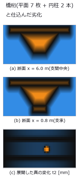
↑ Re-surveying a structure year by year — when the vantage moves, decay appears to advance ―― A bridge girder (7 planes + 2 cylinders) carries known deflection, section loss, bearing settlement and a crack across three epochs, re-scanned each time from different positions, densities and poses. Re-measuring with zero deterioration already yields a nearest-neighbour "change" of 21.07 mm median and 42.64 mm max, and the false repair volume above a 1 mm threshold (5.098 L) reaches 87 % of the real one (5.882 L). Registering on all points absorbs 0.689 of the mid-span deflection (closed form 2/3) and invents a -1.737 mm uplift at the supports, while the undetermined along-span direction shows up not on the girder planes but only on the bearing cylinder, as a spurious 41.2 mm horizontal shift.

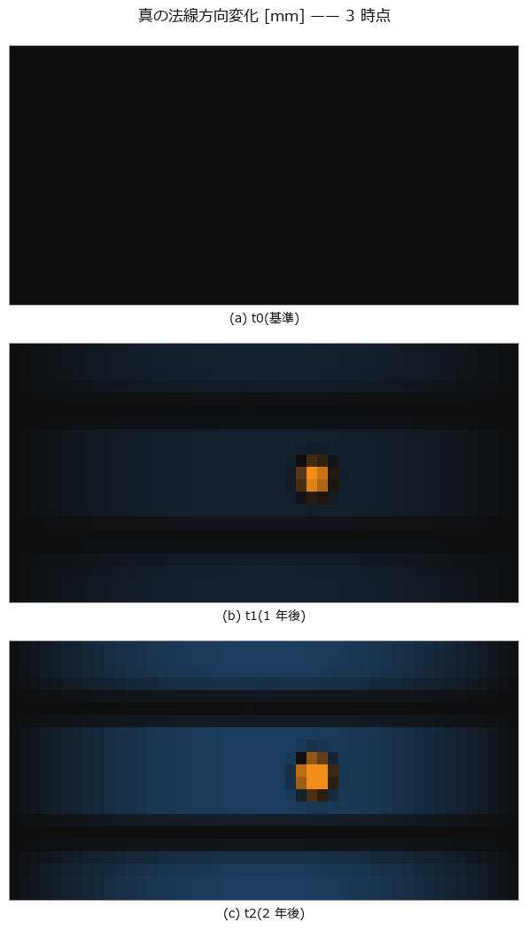
↑ The measurement ―― 下フランジの暗い窪みが断面欠損、面全体の淡い変化がたわみ。腹板(法線が水平)にはたわみが出ない ——同じ劣化でも面の向きで見え方が変わる。 (figure labels are in Japanese; the numbers are the same)

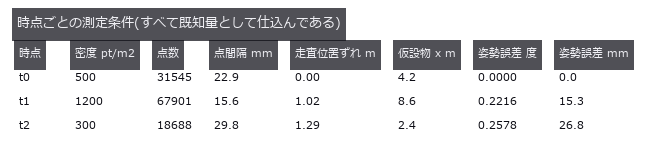
↑ 同じ構造物を 3 回測る。

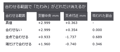
↑ 真のたわみは中央 3.00 mm。

↑ 予測は (ω×(p-c))·n を core 上で積んだだけ。

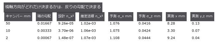
↑ 押し出し形状の平面は法線に x 成分を持たない。

py -3.11 examples/poc_structure_4d_deterioration.py

Source: examples/poc_structure_4d_deterioration.py

This run produced 11 figures in total - see them all

Ops used (notes): box_sdf · chamfer_distance · cylinder_sdf · estimate_normals · euclidean_cluster · fit_circle_3d · fit_plane_3d · grid_coords · hausdorff_distance · plane_sdf · rmse · sdf_intersect · sdf_union · voxel_grid_downsample

No.2026.087 —— Restoring what is missing by symmetry — the plane you assume is the lie you get

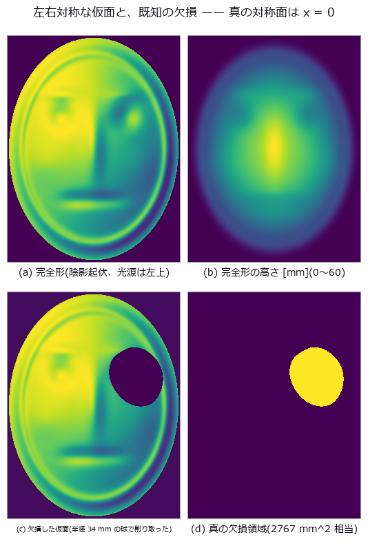
↑ Restoring what is missing by symmetry — the plane you assume is the lie you get ―― A bilaterally symmetric mask is synthesised so that both the complete shape and the true mirror plane are known, then one side is broken off with a sphere. With the true plane, symmetric restoration reaches 0.81 mm RMS and beats harmonic hole filling (1.60 mm) — but it loses the moment the plane is off by 1.39 deg (84 arcmin) or 1.41 mm. The error is predicted by the surface-normal component of the mirror displacement (4.6 % relative error; the naive 2d sin a misses by 50.6 %), so the cliff follows from geometry alone. Losing 3.1 % of the points already flips the PCA candidate ranking onto a 90-degree-wrong axis, and on a shape that is not truly symmetric the restoration fabricates 3436 mm3 of ornament or erases 3495 mm3 — even with the exact plane.

↑ The measurement ―― 失われた真値の点から復元点群までの距離(符号なし、6 mm で頭打ち)。対称復元だけが眼窩の形を取り戻す。 (figure labels are in Japanese; the numbers are the same)

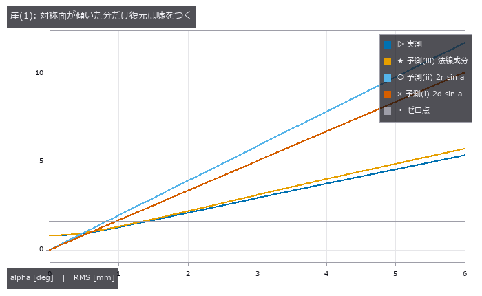
↑ 崖は alpha = 1.39 deg(84 分角)。

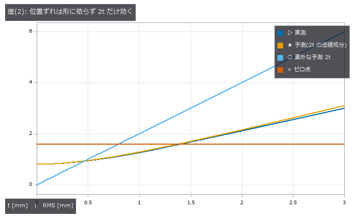
↑ 鏡像点は厳密に 2t 動くが、表面誤差になるのはその法線成分(|n.x| の RMS = 0.50)だけ。

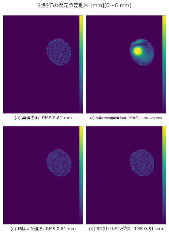
↑ 欠損のまま推定した面で復元すると、欠損部の全体が一様にずれる(位置ずれの署名)。

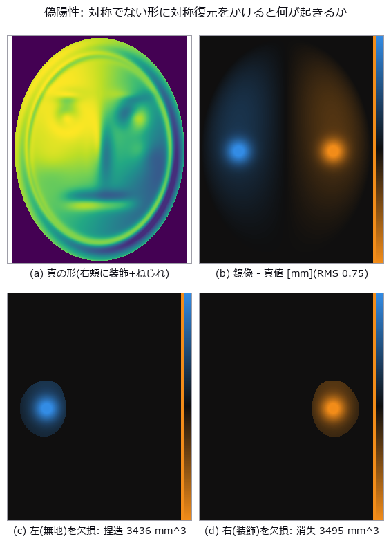
↑ 色は「鏡像 - 真値」。

py -3.11 examples/poc_symmetry_restoration.py

Source: examples/poc_symmetry_restoration.py

This run produced 10 figures in total - see them all

Ops used (notes): detect_reflection_symmetry · fill_holes · fit_plane_3d · icp_point2point_3d · normalize · reflect_points · reflection_symmetry_score

No.2026.146 —— Endless Zooms and Turning Solids: Making the Return Itself the Ground Truth

↑ Endless Zooms and Turning Solids: Making the Return Itself the Ground Truth ―― Motion that never ends still carries equations you can score without watching it end: an infinite zoom returns to the identical picture once you have zoomed by the self-similarity ratio, and a rotating solid returns after 2 pi. Neither loop is made by cutting back to the first frame; both follow from the construction, so the truth is exactly zero difference. The material is Pascal's triangle mod 2 - the same truth that rule 90 satisfies - and the hierarchy of its gaps has a closed form: with I = floor(u2^D), J = floor(v2^D) and b the position of the highest set bit of I & J, the depth is d = D - b. Halving u shifts I right by one, so b drops by one and d rises by exactly one, which is why zooming never costs resolution: every pixel is decided by an integer bit test rather than by magnifying a raster. Over a loop that zooms eight-fold, frame(T) and frame(0) differ by 0.0e+00. The first core finding is that the measured dimension does not move at all under zoom: the existing fractal_dimension operator returns the same value across six zoom levels with a standard deviation of exactly zero, and where the depth of the approximant matches the pixel grid it equals log2(3) = 1.584962500721 to within 8.9e-16 - an agreement, not an approximation. The second is that the same operator returns 0.0 when handed an approximant finer than the pixels; that zero does not mean there is no structure, it means the structure is finer than the sampling, and indeed the level-9 approximant has zero foreground pixels out of 262,144. The third is that 2 pi does not close in floating point: building the rotation from the angle 2pii/T leaves 1.40e-12 in the normals at i = T because sin(2 pi) is -2.45e-16, while closing the period on the integer index instead gives exactly zero. The fourth is a prediction that was wrong and has been left in: the silhouette area of a cube under orthographic projection is a^2(|cos| + |sin|), and the measured two per cent residual was read as the bevel that marching cubes puts on the corners - but pushing the camera from a distance of 6 to 96 dropped the residual from 0.128 to 0.004 for the exact cube and the marching-cubes cube alike, so the floor was perspective, not the mesh. The bevel shows up instead in a quantity that distance does not fix: the ratio of maximum to minimum silhouette area converges to sqrt(2) = 1.4142 for the exact cube but stops at 1.3958 for the extracted surface. Separating one residual into two causes came from sweeping the distance. Two smaller findings: the four-fold symmetry of the depth field is exact while the rendered image breaks it by 1.1e-16, which is the order of summation in a 2x2 average rather than any mathematics; and the two labyrinths of the gyroid have a volume ratio of 0.500000000000, which follows from the odd symmetry. No new operator was added.

↑ The measurement ―― 右は 2 枚の差をそのまま出したもので、全画素が 0(最大差 0.0e+00)。倍率を 8 倍にしたのに同じ絵になるのは、色の巡回(周期 3)が深さの巡回とちょうど噛み合うから。 (figure labels are in Japanese; the numbers are the same)

*↑ *空隙の深さ(色 = 深さ、深いほど濃い)。

↑ 左から深さ 5..9。

↑ 正射影ならシルエット面積は a²(|cosθ| + |sinθ|) で、45 度が最大(√2 倍)。

↑ 厳密な立方体は √2 = 1.4142 に収束する(1.4167)のに、marching cubes で取り出した面は 1.3958 で止まる。

↑ The animation ―― 止めどきは呼んだ側が決める。24 コマで 1 周(8 倍)、そこから先は同じ絵が続く。

↑ The animation ―― 1 周 18 コマ。添字の剰余で角度を作っているので、18 コマ目は 0 コマ目と画素単位で同じ。

py -3.11 examples/poc_endless_zoom_and_turning_solids.py

Source: examples/poc_endless_zoom_and_turning_solids.py

This run produced 15 figures in total - see them all

Ops used (notes): fractal_dimension · gyroid_isosurface · mesh_volume · perpetual_loop_seam · phong_shade

No.2026.149 —— Scoring Four-Dimensional Claims with Ordinary Three-Dimensional Operators

↑ Scoring Four-Dimensional Claims with Ordinary Three-Dimensional Operators ―― The topology and algebra of four dimensions can be scored exactly by ordinary three-dimensional operators already in the box: fitting a circle to a point cloud, the signed volume of a closed mesh, tube meshing and rasterising. The Hopf fibration splits the three-sphere into circles indexed by points of the two-sphere: viewing a point of S^3 as a pair of complex numbers, the fibre over a point of S^2 is the circle q(t) = (cos(theta/2) e^{it}, sin(theta/2) e^{i(t+phi)}), and stereographic projection carries it to an exact circle in space - a Villarceau circle. The first finding is that a four-dimensional circle becomes a two-dimensional point: pushing one fibre through the Hopf map leaves a spread of 8.9e-16 on the sphere, so all 256 sampled points collapse onto one. The second is that the circle-fitting operator recognises it: the projected radius ranges from 0.70 to 7.34 across latitudes, yet the fit residual and the departure from a single plane both stay in the 1e-14 range - a theorem, not an approximation. The third is that two distinct fibres always link exactly once, that the integer emerges from the Gauss integral, and that even the rate of convergence is predictable: doubling the discretisation divides the error by exactly four, measured at 4.01, 4.00, 4.00 and 4.00, confirming the predicted second order. The fourth concerns rotation: in four dimensions a rotation acts in two planes at once, and the motion closes only for rational ratios. A tesseract - 16 vertices, 32 edges, 24 faces, 8 cells, Euler characteristic exactly 0, hypervolume exactly 16 for edge 2 - turned simultaneously in the xy and zw planes returns after sixty steps for ratios 1:2, 2:3 and 3:4 with a difference of 0.0e+00, while the minimum separation along the way stays above 0.23, so it is not the trivial case of nothing having moved. For the golden ratio, refining the step to 400 and running twenty thousand steps still leaves a minimum separation of 0.0257. The period closes because the angle is built from an integer remainder rather than accumulated arithmetic. The fifth finding separates two sources of error in the volume of a tube. Writing two closed forms - one for a circular cross-section on a circular centreline, one for a regular m-gon cross-section on a circular centreline - makes the discrepancy against the second completely independent of m: for a fixed centreline the three cross-sections agree to 7.8e-16. The cross-section's own contribution then vanishes as 1/m^2 exactly as its closed form says, with ratios 3.99 and 4.00. One prediction was wrong and has been left in: the centreline's contribution was expected to vanish as 1/n^2, but doubling and quadrupling the sample count divides it by only 2.09 and 4.15, that is as 1/n - and since the perimeter of the inscribed polygon converges as 1/n^2, the residue cannot come from the perimeter but from the thickness at the joints. Consequently neither knob alone suffices: 96 sides alone stalls at -0.001588 and 1600 centreline points alone at -0.003064, while turning both reaches -0.000925. No new operator was added.

↑ The measurement ―― ホップ束の繊維 4 本を立体射影して管にしたもの。★4 次元では 4 本とも同じ大きさの円なのに、3 次元へ写すと大きさが変わる —— それでも fit_circle_3d は 4 本すべてを 残差 1.4e-14 で円と認める。どの 2 本も必ず 1 回だけ絡む。 (figure labels are in Japanese; the numbers are the same)

↑ fit_circle_3d に 200 点を食わせた残差。

↑ ガウスの積分で求めた絡み数の、整数 1 からの差。

↑ 真値 B は「正 m 角形断面・円中心線」の体積。

↑ 断面の効果は閉形式どおり 1/m²(比 3.99 / 4.00)で消えるのに、中心線の効果は 1/n(比 2.09 / 4.15)でしか消えない。

↑ The animation ―― 同じ 4 本を視点だけ回して見たもの。★視点の周期は角度でなく整数の剰余で閉じている(24 コマ目が 0 コマ目と同じ式になる)ので、継ぎ目が出ない。絡み方は視点を変えても変わらない —— 絡み数は位相の量だから。

↑ The animation ―― 比 1 : 2(有理)。60 コマでちょうど元に戻る —— 戻ったときの差は 0.0e+00。★角度は整数の剰余で作っているので、有理な比なら継ぎ目が出ない。描いているのは 4 次元の超立方体を2 枚の面で同時に回してから w を落とした影。辺は 32 本とも同じ長さなのに、影では伸び縮みする。

↑ The animation ―― 比 1 : φ(無理、黄金比)。この 60 コマでは戻らない。別に刻みを 400 に細かくして 20,000 歩まで回しても、最小の隔たりは 0.0257 で 0 に落ちない。★角度は整数の剰余で作っているので、有理な比なら継ぎ目が出ない。描いているのは 4 次元の超立方体を2 枚の面で同時に回してから w を落とした影。辺は 32 本とも同じ長さなのに、影では伸び縮みする。

py -3.11 examples/poc_four_dimensions_by_three_d_tools.py

Source: examples/poc_four_dimensions_by_three_d_tools.py

This run produced 10 figures in total - see them all

Ops used (notes): curve3d_tube_mesh · fit_circle_3d · mesh_volume

---

This museum was built together with Claude Code. I set the questions and the direction; Claude Code did the implementation, the sweeps, the control groups and the adversarial checks. That division of labour is what made it possible to run 53 PoCs and collect their figures in two days. If you want to try it, this invitation link gives you a one-week free trial: claude.ai/referral/0sqPw8E_lw

If even one exhibit was worth your time, a like or a stock helps: the reactions decide which wing grows next, so tell me in the comments which measurement from your own field you would want to see. And if you swapped in real data and the cliff moved, that is the story I most want to hear.