
title: 'Self-Driving Demos Move, So Nobody Measures Whether They Are Right — A PoC Series Scored by Theorems and Second Implementations'
tags:
- Python
- NumPy
- 自動運転
- アルゴリズム
- robotics
public_private: false
public_id: 05de90f4d316cd7c681c
Language: 日本語 · English
Self-Driving Demos Move, So Nobody Measures Whether They Are Right — A PoC Series Scored by Theorems and Second Implementations

↑ The car (orange) follows the Hybrid A path into the gap: 30 forward segments, 12 reversed, 8 gear changes. You can see that it got in. You cannot see how far this path is from the lower bound.*
About this article
A car backs into a parallel-parking bay. It finds the lane and follows it. It keeps its distance from the car ahead. Self-driving demos move, and nobody checks whether a thing that moves is right.
If the path is not the shortest, the car still ends up in the bay. If the time to collision is overestimated by 20 %, the car still stops in most scenes. If the lane curvature is off by 10 %, the overlay still looks like it hugs the line. The error does not show in the motion — that is what makes this field hard to write about.
So the bar for adding self-driving code is three questions:
(i) Is there a theorem to use as the gate? (ii) Is there a second implementation, one that assumes nothing about the closed-form structure, to use as ground truth? (iii) Is there a published value (an official dataset metric)?
Nothing that fails all three gets written. Checking an answer with the formula that produced it is forbidden.
This series lines up the ops built on that bar, one per instalment. Every instalment ships a moving figure and a score sheet. No trained models: numpy and scipy only, so every number reproduces on your machine. The code is in fullseye and every figure is the script's own output.
Where the series stands
| # | What is measured | Gate (where the truth comes from) |
|---|---|---|
| 1 | How a car turns shortest | Dubins / Reeds–Shepp theorems / forward integration / SLSQP second implementation / Hybrid A* = closed form on an empty grid |
| 2 | The driving school opens — build the world that carries its own truth first | Closed-form areas from the regulation sizes / closed-form ray hits on a plane / two sensors, one world / two point-in-polygon implementations |
| 3 | Time to collision and safe distance — optical-flow τ and the RSS closed forms, scored by the driving-school world's truth | Closed-form τ from depth + rigid motion / the one-frame identity / published RSS parameters and test values / Lemma 2 = worst-case integration |
| 4 | Widening the world — closed-form terrain, world-space materials and procedural trees and pedestrians win the focus of expansion back from flow | Perlin's theorem (zero at lattice points, period, analytic derivative) / fBm spectrum β = 2H + 2 / point–segment distance is eikonal / divergence-theorem volumes / rendered depth back-projected to the world / pure-translation flow radiates from the FoE (true flow = motion) |
| 5 | Giving the car inertia and slopes — stopping just before the line with reaction and braking distance, and a hill start without rolling back | Closed-form stopping distance / RSS stopping distance (second implementation) / closed-form hill-start roll-back / energy balance / notice No. 12 deductions |
| 6 | Sun and weather — when the morning sun hides the signal, how fast you may drive in fog, wet roads and headlamps at night | NAOJ published values / shadow = h cot(elevation) / closed-form veil and chromaticity threshold / Koschmieder's law / road-design manual stopping distance (second implementation) / headlamp performance in the safety standard |
| 7 | An endless map — tiles made around the car, far tiles dropped, 50 km without a break | both sides of a seam agree / regeneration fingerprints (SHA-256) / position re-summed as rationals / the (2r + 1)² bound |
| 8 | Moving traffic and blind spots — a child behind a parked car, meeting oncoming traffic, a bus stop, bad drivers, a pedestrian waiting at a crossing | closed-form sight lines / IDM equilibrium gap / ∫λ and Adams' formula / the habits and intents given (truth) / the Rules-of-the-Road ledger |
| 9 | Decision scenes — checking the rear left in the mirror, predicting amber from the pedestrian light, giving way to an ambulance, waiting for a bus to pull out | Fermat point on the mirror / polygon of edge rays / the signal timing / closed forms for GHM and the stop line / emission-time geometry / arts. 40 and 31-2 |
| 10 | Lateral motion — slowing before a bend, staying in the lane, keeping left for a left turn, not catching a cyclist with the inner rear wheel | friction circle and the ordinance / 2-DOF steady offset / off-tracking closed form / the Rules' positioning / sample gate (0.1 % points and KS) |
| 11 | Level crossings and right of way — stop just before and look both ways, never enter while the alarm sounds or when the far side is blocked, give way to the wider road | railway timing standard / barrier state machine / sight triangle / arts. 36, 38, 44, 50 verdicts / 1 mm grid zones |
| 12 | Overtaking and what you cannot see — wait while the sight distance is short, return once the car shows in the rear-view mirror, do not obstruct the ring, and curve mirrors make cars look far away | zones by brute force over the text / time marches / sight-distance table / 3-D mirror ray tracing and Coddington |
| 13 | Humanoids on the crosswalk — keep the car's physics exact, draw the walkers cheaply | grounded every frame and no stance-foot slip / decimation shift ≤ √3·cell / IoU against direct rendering / hidden behind a nearer wall |
1. How a car turns shortest
Recipe
two poses (x, y, θ) → relative frame → closed-form segment lengths per word → forward-integrate every candidate to verify the endpoint → take the shortest
with obstacles: A* over {left, straight, right} × {forward, reverse} on an occupancy grid, trying a closed-form shot from each node to the goal
A front-steered car has a minimum turning radius ρ and cannot turn tighter. Under that constraint the shortest path from pose (x, y, θ) to pose (x', y', θ') is known as a theorem.
| Term | In plain words |
|---|---|
| Dubins (1957) | For a car that only drives forward the shortest path is arc–line–arc, and the ordering (the word) is one of LSL / RSR / LSR / RSL / RLR / LRL — six, no more |
| Reeds–Shepp (1990) | Allow reversing and the shortest path has at most five segments from 48 words (46 suffice, Sussmann and Tang 1991). Segment lengths are closed form |
| Word | The sequence of segments. L = full left, S = straight, R = full right. Lower case means reversing |
| Occupancy grid | The ground cut into cells, each marked obstacle or free |
| Hybrid A* (Dolgov et al. 2010) | A* over continuous poses, pruned per discrete cell (x, y, θ). The practical answer when obstacles exist |
| Admissible heuristic | An estimate of the remaining cost that never exceeds the truth. The obstacle-free Reeds–Shepp length is one |
| Analytic shot | Trying, mid-search, whether the closed-form path from here to the goal is collision-free. If it is, the search ends |
There are three ops.
-
car_dubins_path(poses, radius)— forward only, six closed-form words. -
car_reeds_shepp_path(poses, radius)— reversing allowed, 48 words (the same 44 formulas as OMPL). -
car_hybrid_astar(occupancy, poses, radius, cell, footprint, ...)— Hybrid A* on an occupancy grid, with a rectangular body or a clearance, and penalties for reversing, gear changes and steering changes.
The closed-form ops forward-integrate every candidate and verify that it reaches the goal; a candidate that misses is discarded and counted in n_rejected. A copying error in a formula does not raise — it shows up as a number.

↑ The six words for one pair of poses. Five reach the goal here; the shortest is the answer. The theorem only says "the answer is one of these six", so all six are built and measured.
Gates and scores
The only ground truths used are theorems, a second implementation and a lower bound. No trained model, no external planner.
| Claim | Measured | Where the truth comes from |
|---|---|---|
| Every closed-form candidate reaches the goal | 0 rejected over 400 random pairs, 6.6 RS candidates per pair (3–12) | Forward integration |
| All 48 words are alive | All 18 word families appear both as candidates and as the optimum | Counting families |
| The closed form really is shortest | Matches the second implementation to 1e-6 on 3 pairs × RS / Dubins (6 cases) | SLSQP over the segment lengths of each word (assumes nothing about the closed form) |
| The theorem's inequalities and symmetries | distance ≤ RS ≤ Dubins, reversibility, reflection, rigid motion, scaling with ρ, triangle inequality — all hold on 400 pairs + 200 triples | Theorem |
| What reversing buys | Dubins − RS at most 10.647 m (ρ = 1 m) | — |
| An aligned goal | Dubins 5.000000 = RS 5.000000, word S. Straight back 2 m: RS 2.000000, word s | Distance is the lower bound |
| Hybrid A* reproduces the closed form | On an obstacle-free grid the cost is 23.353319 m = RS 23.353319 m (1 expansion, first shot). Forward-only equals the Dubins length | Closed form |
| Parallel parking | Cost 16.018 m ≥ lower bound 7.986 m, 3,385 expansions, 42 segments (12 reversed, 8 gear changes), 0.7 s. The poses are collision-free with the body and satisfy |Δθ| ≤ Δs/ρ | Lower bound and kinematics |
| Blocked means refused | Wall the bay off and you get ValueError. No partial path |
Fail-closed |
The second implementation takes the five segment lengths of a word as unknowns l₁…l₅ (signed; negative = reversing), imposes the three endpoint equations (x, y, and the heading as 2 sin(Δθ/2)) as constraints, and minimises Σ|lᵢ| by SLSQP from many random starts, keeping the smallest. It knows nothing about the closed form, so a match rules out both a copying error and a missing word at once.
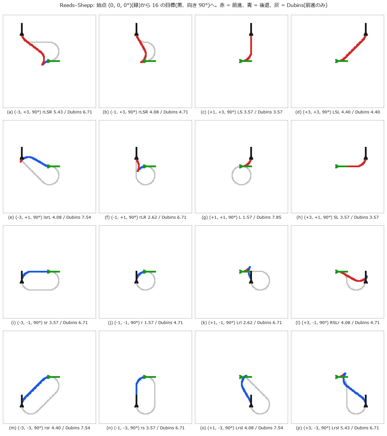
↑ From the origin to 16 goals. Red = forward, blue = reverse, grey = the Dubins (forward-only) path to the same goal. Lower-case letters are reversed segments. With reversing allowed the path is never longer than Dubins.
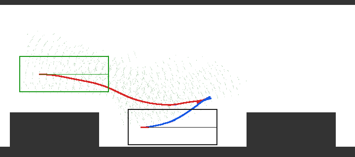
↑ Parallel parking (18 × 8 m, cell 0.25 m, 72 heading bins, body 4.5 × 1.8 m, ρ 5.5 m, a 7.5 m bay). Grey = obstacles (kerb and two parked cars), pale green dots = expanded poses, red = forward, blue = reverse. The obstacle-free Reeds–Shepp path (lower bound 7.986 m) drives through the parked cars, so the cost of 16.018 m is twice the bound. The gap splits into "because of the obstacles" and "because of the pruning approximation", and the two cannot be separated (see below).
★ Where you will get it wrong
Anyone who writes this pipeline will step into four holes. None raises an exception and the car drives plausibly in every one, so without a gate you will not notice.
1. Fold mod 2π the wrong way and eight words never appear
The 44 Reeds–Shepp formulas are normally copied from OMPL. OMPL's mod2pi folds into (−π, π]. Copy them into an implementation that folds into [0, 2π) and the condition t ≥ 0 on a segment length becomes always true: the eight CCSC words (LRSL, LRSR and their symmetric images) never appear as candidates. A negative segment length turns into a detour of 2π − |t|, so you still get an answer and it still reaches the goal — it just is not the shortest.
A gate that asks "does each candidate reach the goal?" cannot catch this, because it does. Only a family-counting gate — group the 48 words into 18 families and demand, over random poses, that every family appears both as a candidate and as the optimum — brings it out. Eight families at zero over 400 random pairs means dead formulas.
2. Write four endpoint equations and the optimiser will not converge
If the second implementation states endpoint agreement as four equations — x, y, cos θ, sin θ — the problem is over-determined (five unknowns, effectively three constraints, four equations) and SLSQP returns infeasible or inf. Write the heading agreement as one equation, 2 sin((θ_end − θ_goal) / 2). Never make both sin and cos equalities.
3. Collision checking eats 80 % of the time
A naive Hybrid A* takes tens of seconds for one parallel-parking run. Profile it and collision checking is 80 %. Three things work: (a) sample the rectangular body, transform all samples to grid coordinates at once, and look them up through a flat index flat[iy·W + ix]; (b) collision-check only the shortest analytic candidate, not all of them; (c) shoot more often near the goal (once every ⌈h / step⌉ expansions for a node with cost-to-go h). Together, 37 seconds become 1 second. Do (a) first — (b) and (c) do not change correctness, which makes their effect hard to measure in isolation.
4. "Unreachable" is sometimes the right answer
Discretisation changes the answer. A 6.5 m bay (car length + 2.0 m) was unreachable at cell 0.25 m with 72 heading bins; a 7.5 m bay is reachable. On a narrow 12 × 8 m grid, a forward-only (Dubins) path leaves the grid, and unreachable is the correct result. In both cases the op raises ValueError. Refusing is safer for whatever runs downstream than returning a partial path that looks like a near miss. If you keep the gate "exact match with the closed form on an empty grid", you can tell whether an unreachable result is the discretisation's fault or the implementation's.
What it is bad at
No moving obstacles and no speed. This is geometry only — which path — and when and how fast to drive it is another layer. Planning around pedestrians and oncoming traffic is a different tool that adds a time axis on top of this op.
Hybrid A is not optimal.* Pruning per discrete cell introduces an approximation, so there is no guarantee that 16.018 m is the shortest path among the obstacles. Of the 8 m gap to the lower bound of 7.986 m, the obstacle part and the approximation part cannot be separated. All that can be said is "at or above the lower bound, collision-free, kinematically feasible" — and that is what the score sheet says.
Curvature is not continuous. Both Dubins and Reeds–Shepp switch the steering instantly at segment boundaries. A real car needs clothoid joins (CC-steer) or downstream smoothing.
Large grids are slow. This is pure-Python heapq; do not use it for 100 × 100 m at cell 0.1 m. It is for ground truth in research, small car parks and teaching.
Run it
git clone https://github.com/furuse-kazufumi/fullseye
cd fullseye
py -3.11 examples/poc_car_parking.py            # 7 gates and 5 figures, about 16 s
import numpy as np
import fullseye as fs

poses = np.array([[0.0, 0.0, 0.0],            # start (x, y, θ)
                  [4.0, 3.0, np.pi / 2]])     # goal
rs = fs.ledger.car_reeds_shepp_path(poses, radius=1.0)
print(rs["word"], round(rs["length"], 4), rs["n_candidates"], rs["n_rejected"])
# LSL 5.1763 9 0     ← word, length [m], surviving candidates, candidates the integration rejected (if not 0, suspect the formulas)

occ = np.zeros((32, 72), bool)                # 8 × 18 m at cell 0.25 m
occ[:2, :] = True                              # kerb
res = fs.ledger.car_hybrid_astar(occ, np.array([[2.0, 4.2, 0.0], [7.5, 1.5, 0.0]]),
                                 radius=5.5, cell=0.25, footprint=(4.5, 1.8, 1.0))
print(res["cost"], ">=", res["lower_bound"], res["n_expanded"])
Always look at n_rejected. A non-zero value does not mean your poses are bad — it means a formula somewhere is dead.
This instalment produced 5 figures in all — see them all
The remaining figure of this instalment

↑ All 11 ground truths: 6 from the second implementation, 3 aligned goals, 2 empty grids. Every point sits on the diagonal.
2. The driving school opens — build the world that carries its own truth first

↑ A chase camera with the LiDAR (16 beams) points overlaid. Grey = road, yellow = kerb, red = car, green = signal, white = crosswalk. The box at the top right is the in-car camera's ROI and its verdict — the car waits at the stop line while it reads red and moves on the frame after it reads green (closed loop). Red light → intersection → crank (with reversing) → link road → loop. That the car drove is visible. How many centimetres its corners crossed the kerb line, and which face every LiDAR point came from, is not — but the world knows, so it can be counted.
Part 1 had only the geometry of paths; there were no sensors. To score a sensor you need a world in which what it sees is decided in advance. The ground truth of real datasets is human labelling: the edge of every box and the label of every point is somebody's judgement. So this part builds the world instead — not with arbitrary sizes, but with the numbers of Appendix 3 of the Road Traffic Act Enforcement Regulations (standards for designated driving-school courses, ordinary licence).
Recipe
regulation sizes → one polygon per element (crank, S-curve, slope, parallel parking, turnaround, level crossing, loop, main roads)
       → place with (x, y, yaw) → union = drivable region
       → 3-D world: ground plane + kerb bands + lane paint + crosswalks + stop lines + CC0 cars + signals and signs generated procedurally to Japanese standards (every face carries a label and a colour)
       → read the signal colour from the in-car camera image (map position → ROI → chromaticity detection) and do not move until it reads green (closed loop)
       → fire a spinning LiDAR at the mesh (points, range image, face labels) / render the in-car camera (colour, label, depth)
       → drive it with round 13's Hybrid A* and score every pose and every frame
| Term | Meaning here |
|---|---|
| Loop course | Oval. Straights ≥ 80 m, width ≥ 8 m. The outer ring of a driving school; the exercises sit inside it |
| Main roads | Roads ≥ 7 m wide crossing at right angles and joining the loop. Corner radius ≥ 3 m |
| Crank | 3.5 m wide, 12 m between the bends, entries ≥ 4 m, 1 m fillet on the inner corners (ordinary licence) |
| S-curve | 3.5 m wide, 7.5 m radius (outer arc), two arcs of 3/8 of a circle in opposite senses |
| Turnaround | A 3.5 m bay, 5 m deep, beside a 3.5 m road, 1 m fillets |
| Slope | ≥ 7 m wide, ≥ 1.5 m rise, gentle grade 6.5–9 %, steep 10–12.5 %, ≥ 4 m flat top |
| Range image | One LiDAR sweep on a grid: row = elevation (beam), column = azimuth, value = range |
| Inverse sensor model | The rule that turns "a return came back at this range" into occupancy updates of grid cells (here: just dropping kerb points into cells) |
The new ops live in three modules. drivecourse (regulation-size 2-D polygons; truth = closed-form areas), driveworld (the 3-D world; CC0 Kenney Car Kit / City Kit Roads meshes for cars, street lights and cones scaled to real dimensions, and signals and signs from roadjp, generated procedurally to Japanese standards: a horizontal three-lamp head with green, yellow, red from the driver's left, hung from an arm on a pole at the far side of the intersection with the lamp bottom at 5.0 m; signs as a 600 mm circle, a 600 mm inverted triangle, a 450 mm warning diamond, plate bottom at 1.8 m; the camera image is looked up from triangle ids), and lidarsim (Möller–Trumbore ray–triangle intersection, accelerated by binning every triangle by the azimuth and elevation intervals it subtends from the sensor; 80 k triangles × 58 k rays in under a second).

↑ From above. The loop (80 m straights, 8 m wide, R 30 semicircles) with the cross of main roads inside (four signals, a crosswalk on each arm and a stop line 2 m before it). Crank to the north-east, S-curve south-west, slope south-east (the dark patch is the ramp), parallel parking and turnaround north-west, level crossing on the eastern main road. The exits rejoin the loop through link roads, so you can circulate.

↑ The 3-D world. Kerbs (0.15 m) and lane paint follow the polygon edges and are left out at the joints. Cars, street lights and cones are CC0 meshes; the signals (horizontal three-lamp heads on arms over the lane, from the far-side pole) and signs (stop, slow, speed limit, crosswalk, level crossing ahead) are generated procedurally to Japanese standard dimensions. Every face has a label and a colour.
Gates and scores
Three kinds of truth: closed forms derived from the regulation sizes, closed-form ray hits on planes and boxes, and the identity between two sensors looking at one world. No trained model and no external simulator.
| Claim | Measured | Where the truth comes from |
|---|---|---|
| The polygons are the regulation sizes | For the 5 elements with arcs, the shoelace area converges monotonically to the closed form as the arc goes 16 → 64 → 256 → 1024 points (crank 3.1e-5 → 7.5e-9, S-curve 2.8e-3 → 6.8e-7). The 4 arc-free elements match exactly | Closed forms (crank = w·L + 2r²(1 − π/4), S-curve = 2·(3/8)·π·(7.5² − 4²) + entries, semicircle = π R w) |
| The LiDAR measures a plane correctly | 10,903 points on flat road: range vs h/(−sin e), relative difference 2.1e-16 | Closed form |
| The two sensors see one world | 3,450 LiDAR points projected into the camera: median relative depth difference 2.9e-3, label agreement 100 % (1-pixel tolerance; 99.1 % pixel-exact) | Identity |
| Car points are inside cars | 1,607 points labelled "car" lie inside the placed car boxes (pose + real size): 100 % | The world's own placement |
| Kerb points are off the road | An occupancy grid built from 4,667 kerb points is a subset of the true occupancy (outside the polygons) dilated by one cell (precision 1.0000), in all 68 driving frames | Point-in-polygon (two implementations: even-odd and winding) |
| The driven path does not derail | Over 997 poses the corners of the body cross the kerb line by at most 0.117 m ≤ half a cell (0.125 m); on the exact polygons 11 poses cross (the planner's resolution) | Polygons |
| Zero point | Driving the crank in a straight line derails in 50 of 60 poses | — |
| The camera reads the signal (image processing) | The lamps' map positions are projected into the in-car camera; a chromaticity detector searches the ROI (± 24 px) for lit discs. Red → red, green → green, lamps off → unknown. No ground-truth face ids are used |
The world's own state |
| No motion until it reads green (closed loop) | From the stop line the camera is read every frame and the car moves on the frame after it reads green. During the 6 red frames it does not move a millimetre; the 11 readings from 10 m out all match the world's state. Zero point: with the lamps off it keeps reading unknown and does not start in 8 frames |
The world's own state |

↑ A sweep 10 m before the stop line (32 beams, −25° to +15°, 0.5°; 10,903 points on the road). Points are coloured by the label of the face they hit — that this is generation-time truth rather than human labelling is the whole value of the world.

↑ The same instant from the in-car camera (60°, 640 × 400) with the LiDAR points projected onto it. Point depth vs pixel depth and point label vs pixel label agreeing is the "two sensors, one world" gate. The signal is red.
★ Where you will get it wrong
1. The regulation 3.5 m width cannot be driven forward with max-steer-and-straight primitives
Part 1's Hybrid A* uses {left, straight, right} × {forward, reverse} motion primitives. With a 4.5 × 1.8 m car, the regulation crank (3.5 m wide, 1 m fillets) is unreachable forward-only — at 0.25 m cells with 72 heading bins and at 0.125 m with 144 — the search exhausts its open set after a few dozen expansions. The S-curve (outer 7.5 m, inner 4 m) is the same. Allowing reversing gets through (crank: cost 57.9 m, 14 reverse segments; S-curve: 29.5 m, 1). The real driving test allows reversing too, with points deducted per manoeuvre. Without intermediate steering angles in the primitives, a corridor that fits geometrically does not fit after discretisation — the opposite of "it moved so it is right": it did not move, and that was not wrong.
2. "Collision-free" from the planner still pokes 12 cm over the polygon
Collision checking is per cell (0.25 m). Measured on the exact polygons, 11 of 997 poses have a body corner over the kerb line, by up to 0.117 m. That is within half a cell, so the planner kept its promise — but "collision-free" is only as strict as the resolution. The gate sits at half a cell and reports the number of crossing poses and the largest excursion. If you must not touch the kerb, add clearance or refine the grid; both cost time.
3. Elements that touch edge to edge grow a kerb wall across the joint
If the loop's straights and semicircles meet exactly on a shared edge, neither end edge is "inside the neighbour", so both grow kerbs — a wall across the road. The LiDAR saw it and dropped kerb points into cells that should be drivable (precision 0.90). Two fixes: overlap adjacent elements by 5 cm, and skip a 0.5 m edge piece if either endpoint or the midpoint lies inside a neighbour. Testing only the midpoint leaves pieces half across a mouth, and they become walls.
4. A signal beside the stop line is outside the stopped car's camera
At first the signal stood beside the stop line. From the stopped car the in-car camera (60°, looking 20 m ahead) would have to look 40° up to see the lamps. Japanese vehicle signals go on the far side of the intersection (the signal installation guidelines), and from there the lamps are 18 m away at 9° elevation and readable. Position and height are standardised — a horizontal head on a 1.5 m arm with at least 5.5 m from ground level (prefectural police works specifications), sign plates with the bottom edge at 1.8 m and at least 25 cm from the kerb line (the road-sign installation standard). Place things by eye and this is where the world starts lying.
5. Thin objects land on a different face one pixel over
A kerb is 0.15 m tall — a two-pixel band at 20 m. Comparing a projected LiDAR point with the label of the same pixel gives 99.1 %, and most misses are kerb points landing on the neighbouring road pixel. Counting a match if the same label appears in the 3 × 3 window gives 100 %. Lane paint (0.12 m wide) is under one pixel far away, so it is counted as the road surface it is painted on. Writing "100 % label agreement" without the tolerance in pixels means nothing.
6. Huge triangles vanish behind the camera
Modelling the ground as two enormous triangles makes the road disappear from the in-car camera: the rasteriser drops any triangle with a vertex behind the camera (it does no near-plane clipping by design). A 4 m grid confines the loss to the cell under the camera. The LiDAR has a cousin of this trap: taking a triangle's elevation interval from its vertices' min and max misses the middle of an edge passing over the sensor (an edge between two 5.7° vertices reaches 78.7°). Each edge needs its great-circle extremum added.
What it is bad at
No moving objects and no time. The world is static and the car merely follows a pose sequence. No oncoming traffic with speed, no pedestrians. The signal changes colour but has no rule for when.
Sensor physics is geometry only. The LiDAR has single returns, no intensity, no beam divergence, no rain or fog, no distortion from ego-motion during the sweep. The camera is Lambert shading only, no shadows, no exposure. This is not evidence that a detector works on a real car; it is a tool for finding geometric mistakes.
The car meshes have toy proportions. Kenney's CC0 models are stretched per axis to the box dimensions (4.5 m long, 1.8 m wide; within 1.8× of the raw proportions). The point-cloud shapes differ from real cars. The orientation of an asset is not decided by eye: the raw model's longest axis, its left–right mirror symmetry (mirroring the width maps the shape onto itself, mirroring the length does not) and the lamp colours (yellow = headlights, red = tail lights) are gates, and so is the max/min ratio of the per-axis scale factors, because per-axis scaling with the wrong orientation crushes the shape.
Parallel parking has no size in the regulation. The appendix of the circular is a figure and no primary numeric source was found, so the default bay is car length + 3.0 m, and the docstring says so.
Run it
git clone https://github.com/furuse-kazufumi/fullseye
cd fullseye
py -3.11 examples/poc_driving_school.py         # 14 gates and 6 figures, about 37 s
import numpy as np
import fullseye as fs

crank = fs.ledger.course_crank()                                  # regulation: 3.5 wide, 12 between bends, 4 entries, 1 fillet
P = crank["polygon"]                                             # counter-clockwise polygon (K, 2)
area = 0.5 * abs(np.dot(P[:, 0], np.roll(P[:, 1], -1)) - np.dot(P[:, 1], np.roll(P[:, 0], -1)))   # shoelace
print(crank["params"]["regulation"], round(area, 3), round(crank["area_closed_form"], 3))
# {'A': 3.5, 'B': 12.0, 'C': 4.0, 'D': 1.0} 82.682 82.679

world = fs.ledger.world_build(crank, props=[("sedan", 20.0, 2.0, np.pi / 2)])   # make it 3-D and park one car
spec = fs.ledger.lidar_spec(n_beams=16, azimuth_res_deg=1.0)
T = np.eye(4); T[:3, 3] = (2.0, 0.0, 1.64)                        # inside the entry, sensor 1.64 m up
scan = fs.ledger.lidar_scan(world["V"], world["F"], spec, T, labels=world["face_label"])
hit = scan["ranges"] > 0
print(scan["n_hits"], np.bincount(scan["labels"][hit]))
# 2641 [2455  140   22    0    0    0    0    0    0   24]   ← number of points, per face label (road 2455, kerb 140, car 22, …, paint 24)
labels is the label of the face each ray hit. It is generation-time truth, so once you write a detector you can score it against this without waiting for human labels.
This part produced 6 figures in all — see them all
The remaining figure of this part

↑ Areas of the 8 element kinds (shoelace vs closed form) and 200 road ranges (measured vs h/(−sin e)). Everything sits on the diagonal.
3. Time to collision and safe distance — optical-flow τ and the RSS closed forms, scored by the driving-school world's truth

↑ In-car camera, 0 → 10 s. While the oncoming car is in view its pixels carry the optical flow (arrows) and the true focus of expansion (cross), with the "true τ" and the "τ from flow" side by side at the top. After it passes, RSS flags the parked car in the ego lane as dangerous (t = 6.0 s), the ego brakes and stops 10.25 m short. The numbers move because the world holds the truth — τ and gap are not estimates, they are fixed at generation time.
Part 2 built the world, but nothing in it moved. This part sends a car the other way. Two questions: how many seconds until we collide, and how many metres should we keep. The first is Lee's (1976) τ theory — the time to collision with an approaching surface follows from how fast its image grows, with no distance and no speed; flies and humans brake on it. The second is Mobileye's RSS (Shalev-Shwartz et al. 2017) — from a response time and bounds on acceleration it gives, in closed form, the distance below which you are to blame. Both are textbook formulas, and in this world both can be checked against truth.
Recipe
Part 2's loop course (south straight, 80 m, left-hand traffic) → ego 8 m/s (north lane), oncoming 8 m/s (south lane), parked car ahead in the ego lane
   → in-car camera 60°, 640 × 400, 10 Hz, 4.5 s (46 frames)
   → τ three ways: truth (depth image + rigid motion between frames, closed form) / from flow (LK → time_to_contact) / from size (square root of area)
   → RSS: closed-form safe distances with the published parameters → time-integrate the worst case and compare → three school scenes with verdict and braking
| Term | Meaning here |
|---|---|
| τ (tau) | Time to collision. With Z the depth of the surface and Ż its rate, τ = Z / (−Ż). At constant speed it falls one second per second (dτ/dt = −1) |
| Focus of expansion (FoE) | For a translating camera, the image point the flow radiates from — the image of the heading |
| Optical flow | Where each pixel moved between two frames, (u, v). Here pyramidal Lucas–Kanade, 5 levels |
| RSS | Responsibility-Sensitive Safety: the definition and closed form of the distance at which, whatever the other car does within bounds, your prescribed response avoids contact |
| ρ (response time) | Time from the situation becoming dangerous to the start of braking; the worst case assumes you may accelerate meanwhile |
| a_min,brake / a_max,brake | The least deceleration you are guaranteed to apply / the most the other car might apply |
| Proper response | What RSS prescribes: anything up to a_max,accel during ρ, then at least a_min,brake until stopped |
Two new modules. drivettc derives, per pixel and in closed form, the true flow and the true τ from the depth image and the rigid motion; the flow-based τ wraps the existing time_to_contact and converts it to seconds. rsssafety holds the RSS closed forms for same-direction, opposite-direction and lateral distances, the worst-case time integration, and the verdicts. All three τ values are aligned to the time of the first frame — there is a one-frame trap here, described below.

↑ t = 4 s. The flow on the oncoming car's pixels (arrows ×3) points outward from the focus of expansion (cross); its radial speed gives τ = 0.84 s (truth 0.84 s). The road has no texture, so flow exists only on the car and the lamp post.
Gates and scores
Three kinds of truth: closed forms from the depth image and the rigid motion (τ), published values (the RSS parameter table and test values), and a theorem agreeing with an integration (Lemma 2).
| Claim | Measured | Where the truth comes from |
|---|---|---|
| The true flow gives τ back (identity) | Feeding the true flow to time_to_contact and adding one frame matches the true τ₀ to 8.5e-14 (46 frames, every pixel of the car) |
Closed form |
| τ falls one second per second | The car's nearest pixel's τ equals "distance to the front bumper / closing speed" within 8.3e-3, slope −1.0045 | Poses and speeds |
| Flow yields τ | Over the 22 frames where the car covers ≥ 150 px, LK τ has median relative error 0.026 (90th percentile 0.30); over all 46 frames 0.135 | Closed form |
| Size yields τ | From the square root of the area (0.5 s apart), median relative error 0.045 (90th percentile 0.12); the truth lies inside the quantisation band [area ± perimeter/2] in 17 / 19 frames | Closed form |
| RSS closed forms match the published values | ad-rss-lib's five lateral test values within 0.0065 (tolerance 0.01). Same direction at 50 km/h: 39.8 m with no acceleration (published ≈ 40), 83.6 m with 4 m/s² (published "about 80") | Published values |
| Lemma 2 agrees with the worst-case integration | At v = 8 m/s, d_min = 26.28 m; integrating from there the minimum gap is 4.3e-14. Over 50 random parameter sets |min_gap − (d₀ − d_min)| < 1e-13, and collision/no collision agree | Second implementation |
| The school stops in time | Danger at 26.25 m (< 26.28) → speed held for ρ = 1 s, then 4 m/s² → final gap 10.25 m = gap(t_b) − (vρ + v²/2b) to 1e-9 | Closed form |
| τ shouts, RSS does not | For the car in the other lane true τ falls to 0.30 s, yet the lateral safe distance is 0.725 m < the 2.2 m lane gap, and RSS never flags danger | Closed form |
| Drift over and it is dangerous | If the oncoming car drifts sideways at 0.6 m/s the lateral safe distance jumps to 2.45 m and danger starts at t = 1 s; the longitudinal gap of 58.25 m is then already inside the 82.9 m opposite-direction distance, and the worst case collides (minimum gap −24.7 m) | Second implementation |

↑ The two truth lines (overlapping) fall from 5 s at slope −1. Flow-based τ (light blue) sits on the truth from t ≥ 2 s and scatters at range where the flow is below one pixel. Size-based τ (orange) stays close throughout.

↑ The gap to the parked car (blue) drops below the safe distance (orange, 26.28 m at v = 8) at t = 6.0 s: danger. Speed held for one second, then 4 m/s². The safe distance falls with v during braking.
★ Where you will get it wrong
1. τ from a two-frame flow is the τ one frame later
τ = Z / (−Ż) is an instantaneous quantity. With flow from two frames, an image point moves to Z₀/Z₁ times its distance from the focus of expansion, so time_to_contact's "radius² / (radial flow · radius)" is Z₁ / (Z₀ − Z₁) frames — the τ at the second frame, exactly one frame less than at the first. At 10 Hz that is 0.1 s, which is 20 % when τ is 0.5 s. Add one frame and it matches the truth to 1e-13 (gate 1). The difference is one frame even when the speed is not constant, so it suffices to decide which instant your τ refers to and be consistent. The size-based τ has the same one-frame offset (Δt·w₁/(w₁ − w₀) at the first frame, Δt·w₀/(w₁ − w₀) at the second).
2. Flow-based τ works only while the flow is one to a dozen pixels
At range (car under 100 px, flow under one pixel) LK τ is 20–70 % off; too close (flow over 50 px) even five pyramid levels lose track. In between, 22 frames give a median of 2.6 %. Lengthening the frame interval to gain flow sounds right and made things worse here (0.3 s apart: four times the error) — LK assumes appearance does not change, and an approaching car changes appearance. "Flow gives τ" is conditional, and the condition can be written in pixels of flow.
3. Size-based τ loses to area quantisation
Since the square root of the area n scales as 1/Z, τ₀ = Δt / (1 − √(n₀/n₁)). One frame apart (0.1 s) the area gain (30 px at τ = 2 s and 300 px) is smaller than the edge quantisation (half of an 80 px perimeter) and the band opens to infinity. Half a second apart the truth lies inside the band in 17 of 19 frames; the two outliers are the car's silhouette not being planar (its side comes into view as it nears). From the same two frames, flow wants a short interval and size wants a long one — keep separate intervals if you use both.
4. The lateral RSS formula differs in sign handling between the paper and the public implementation
The paper's lemma is written for the case where both cars are still moving toward each other after ρ; outside that case (one is still moving away) the literal formula adds the receding car's stopping distance in the approaching direction. Intel's public ad-rss-lib adds the stopping distance only when the post-response velocity points at the other car, and treats μ differently (paper μ + [·]₊, library [· + μ]₊). The published test values are the library's, so this implementation follows the library and gates that it agrees with the paper inside the paper's assumption (over 100 of 300 random cases satisfy it; agreement to 1e-9). "The paper's formula verbatim" and "the same as the public implementation" are different claims.
5. The closing speed is v cos θ by the camera's pitch
The in-car camera looks slightly down (1.4°). Depth is measured along the optical axis, so the closing speed of the oncoming car is not 16 m/s but 16·cos 1.4° = 15.995 m/s. Writing the truth as "distance / 16" is off by 3e-4 — small, but a 1e-9 gate does not pass. The truth formula must carry the axis direction.
6. The focus of expansion cannot be estimated from flow in this world
A least-squares FoE from the whole flow field lands a median 62 px from the truth: the road has no texture, so flow exists only on the car and the lamp post. This part takes the ego motion as known and supplies the true FoE (reported, not gated). In real footage the road texture is what pins the FoE — a world without texture kills the estimate, a failure that tells you what to add to the world next.
What it is bad at
Ego motion is known. The focus of expansion and the mask of the oncoming car's pixels (the world's face ids, standing in for a perfect detector) come from the truth. This is not a score for a whole perception pipeline with a detector and ego-motion estimation; it scores whether the τ formulas and the RSS formulas agree with the world.
RSS verdicts use two axes only, longitudinal and lateral; intersections, right of way and occlusion (the paper's second half) are not included. The parameters are ad-rss-lib's "initial values for discussion"; neither the paper nor any law fixes numbers.
The oncoming car moves at constant speed in a straight line. τ under deceleration, acceleration or mid-lane-change (dτ/dt ≠ −1) is not covered. The formulas apply as they are, but the "slope −1" gate is a constant-speed property.
The world ends 8 m outside the course and the road surface is plain. No street trees, pedestrians or crosswalks yet — which is also why no flow can be taken from the road.
Run it
git clone https://github.com/furuse-kazufumi/fullseye
cd fullseye
py -3.11 examples/poc_ttc_rss.py         # 10 gates and 6 figures, about 35 seconds
import numpy as np
import fullseye as fs

# τ: one depth image, approaching at 8 m/s for 0.1 s (+z is forward in the camera frame)
K = np.array([[34.6, 0.0, 31.5], [0.0, 34.6, 19.5], [0.0, 0.0, 1.0]])   # 64 × 40, 60° vertical (τ does not depend on K)
depth = np.full((40, 64), 20.0)                                  # a wall 20 m ahead
T = np.eye(4); T[2, 3] = 0.8                                     # 0.8 m closer per frame
truth = fs.ledger.ttc_truth(depth, K, T, 0.1)
flow = fs.ledger.flow_from_depth_motion(depth, K, T)              # the true flow (u, v)
est = fs.ledger.ttc_from_flow(flow["u"], flow["v"], 0.1, foe=fs.ledger.foe_from_motion(K, T))
print(round(float(np.nanmedian(truth["tau"])), 6), round(est["tau"], 6))
# 2.5 2.5                                                         ← 20 m / 8 m/s; identical with the one-frame correction

# RSS: ego at 8 m/s, a stopped car ahead. ρ 1 s, accel 3.5, braking 4 / 8 m/s² (the ad-rss-lib table)
p = fs.ledger.rss_params()
d_min = fs.ledger.rss_longitudinal_same(8.0, 0.0, p)
sim = fs.ledger.rss_worst_case_gap(d_min, 8.0, 0.0, p)
print(round(d_min, 3), round(sim["min_gap"], 9), sim["collided"])
# 26.281 0.0 False                                                ← closed form = integration, exactly zero and no contact
This part produced 6 figures in all — see them all
The remaining figures of this part

↑ The 80 m south straight from above (t = 3 s): ego (north lane, eastbound), oncoming car (south lane, westbound), parked car (x = 40).

↑ In their lanes the lateral gap of 2.2 m exceeds the 0.725 m safe distance, so falling τ (grey) never becomes danger. Once the oncoming car drifts at 0.6 m/s the safe distance jumps to 2.45 m and danger starts at t = 1 s.
4. Widening the world — closed-form terrain, world-space materials and procedural trees and pedestrians win the focus of expansion back from flow

↑ In-car camera, 0 → 10 s (51 frames, 6 m/s). Arrows are Lucas–Kanade flow (×4), the orange cross is the focus of expansion estimated from flow, green is the truth. The road carries grain, puddles and worn lane paint, a pedestrian crosses at the crosswalk, and outside the road there is fBm relief with trees. The numbers at the top are the road grade and the FoE error (all pixels / road only). The focus of expansion that missed by 62 px in part 3 lands within 1–2 px once the road has texture — and because every grain of that texture is a world-coordinate formula, the error can be counted in pixels.
Part 3 ended with two honest caveats. The focus of expansion (FoE) was taken as "known": the road had no texture, flow existed only on the car and the lamp post, and a least-squares estimate missed by a median of 62 px. And the world ended 8 m outside the course. This part widens the world — under one condition: everything added must carry its truth from the moment it is generated.
That condition is the design axis of this series, fixed in part 2 when it switched to building the world instead of borrowing one. Synthetic datasets (Virtual KITTI, SYNTHIA, CARLA) also take labels, depth and flow from a renderer, and those are stricter than human labels. The difference is the kind of truth. A renderer can say which face a pixel belongs to and how far away it is; the height and gradient of the ground, the distance to the road, the wear of a lane marking, the reflectance of a puddle are values baked into a mesh or a texture, not formulas. Here the terrain height, its gradient, the distance to the course, the wear and the reflectance are closed-form fields. When a field is a formula, the rendered image can be projected back onto it and compared with it, and theorems — a spectral law, the eikonal equation, the divergence theorem — become gates. This is the opposite purpose to domain randomization (Tobin et al. 2017), which scatters appearance so that a learner becomes insensitive to it: here appearance is not scattered but derived from fields that hold the truth, for scoring rather than training.
How this differs from prior work. Before starting, I searched my own literature corpus (procedural terrain, road networks, OpenDRIVE, synthetic driving datasets, domain randomization, hard road surfaces; 1,652 OpenAlex papers). Terrain generators are numerous — fBm, Perlin, Weierstrass–Mandelbrot, hydraulic erosion — but no abstract in the corpus states the relation between spectral slope and Hurst exponent as a test; the closest are a 2006 paper that estimates fractal dimension from the slope of a log–log periodogram and a 2023 paper that generates road-surface profiles from a prescribed PSD. Road-network generators (Parish and Müller 2001 with L-systems, Chen et al. 2008 with tensor fields) build streets, but no abstract names clothoids, Euler spirals or paramPoly3 as a checked invariant, and a 2022 validation study of 99 OpenDRIVE datasets found lane gaps in roughly 20 % of them — map geometry usually has no gate at all. Synthetic driving datasets (Virtual KITTI with detection, tracking, semantic and instance labels, depth and flow; SYNTHIA with pixel labels; Playing for Data with semantic labels captured from GTA V; the CARLA-derived SELMA with many sensors and weathers; SynPeDS with pedestrians and safety metadata) all take their labels from a renderer, so nothing in them can be checked against a theorem. Hard road surfaces — puddles (polarisation stereo in 2017, a reflection-attention cGAN in 2019, AGSENet in 2024), worn lane markings, crosswalks (CDSet, 3,434 images), occluded pedestrians — are almost all hand-labelled; the only truth-bearing synthetic sources are a 2025 3D-Gaussian-splatting renderer for rain and reflections and a 2026 Blender puddle set, and no generator synthesises worn markings with a wear truth. The difference here is that every field of the world — height, gradient, distance to the course, wear, puddle reflectance — is a closed-form function, so the gates are theorems and identities rather than agreement with a renderer.
Recipe
relief = sum of random-phase sinusoids (spectral synthesis of fBm, H = 0.8, 1,024 waves, periods 6–120 m) → height and gradient in closed form
   → distance field to the course (point–segment distance, |∇d| = 1 off the road): flat within 2 m of the road, blended into the relief over 12 m → long-wave undulation on the road (±0.8 m)
   → applied after the fact to part 2's flat world (the ground cells are replaced by the terrain mesh; assets are lifted rigidly by the height at their pose)
   → 70 trees (prism + cone / spheroid) scattered ≥ 4 m from the road and ≥ 5 m apart, a crosswalk (9 stripes), a pedestrian (boxes + a solid of revolution), signs, lamp posts, cars, a cone
   → render the in-car camera, back-project each pixel's depth to world coordinates, evaluate Perlin noise there: grain, grass, stains, puddles, worn paint, per pixel
   → LK flow from two frames at 30 fps → least-squares FoE from the road pixels only → compare with the truth; also against the same terrain and trees with the texture removed
| Term | Meaning here |
|---|---|
| fBm (fractional Brownian motion) | A surface that looks equally rough at every magnification. One number, the Hurst exponent H (0–1), sets the roughness; larger H is smoother |
| Power spectrum and β | The strength of each spatial frequency f in the surface. For fBm it is a straight line f^{−β}, with β = 2H + E (E = dimension, 2 for a surface; Saupe 1988) |
| Spectral synthesis | Building the surface as a sum of sinusoids with amplitude ∝ f^{−H} and random direction and phase. A sum is a formula, so height and gradient are closed form |
| Perlin gradient noise | Random gradient vectors on a lattice; the value is "gradient · offset from the lattice point", interpolated with a smooth polynomial (Perlin 2002). The offset is zero at a lattice point, so the value is exactly zero there; the permutation table has 256 entries, so the period is 256; differentiate the polynomial and the derivative is closed form |
| Distance field and eikonal | The shortest distance d(x, y) from a point to the road. Where the nearest point is unique, ∇d is the unit vector pointing away from it, so |∇d| = 1 (the eikonal equation). The terrain uses d to stay flat near the road |
| Divergence-theorem volume | The volume of a closed mesh is Σ v₀ · (v₁ × v₂) / 6. Prisms and polygonal cones match their closed forms exactly; an inscribed spheroid never exceeds its bound |
| World-space material | Texture decided by the world's (x, y), not by image coordinates. The pattern stays glued to the road as the car moves, which is what produces flow |
| Balanced error rate | The mean of the miss rate and the false-alarm rate of a two-class rule. When no threshold brings it down, the classes are genuinely hard to tell apart |
The new ops live in one module, driveterrain (fBm, Perlin, distance field, terrain, materials, trees, pedestrian, crosswalk, scattering, volume). foe_from_flow, which estimates the FoE from flow, was added to part 3's drivettc.
There are only four formulas and all are readable. (1) Relief: h(x, y) = Σ_k A_k cos(2π f_k (x cos θ_k + y sin θ_k) + φ_k). Draw the frequencies f_k log-uniformly and their density in the 2-D frequency plane is ∝ 1/f²; with amplitudes A_k ∝ f^{−H} the power is A² × density ∝ f^{−(2H+2)} — the theorem's β = 2H + 2 falls out directly. The gradient is the sum of the term-wise derivatives. (2) Terrain: z = h · w(d) + undulation, where w is a smoothstep that is 0 up to 2 m from the road and reaches 1 over the next 12 m. The product rule ∇(h·w) = w∇h + h·w′(d)·∇d, with ∇d the normal of the distance field, keeps the gradient closed form. (3) Materials: back-project the rendered depth to recover each pixel's world (x, y) and evaluate Perlin noise there. A puddle is where the noise exceeds a level (label 11); with wear ∈ [0, 1] the paint colour is white · (1 − wear) + road · wear. (4) FoE: under pure translation the flow radiates from the FoE (Longuet-Higgins and Prazdny 1980), so the line through each pixel along its flow direction — its flow line — must pass through the FoE. The FoE is the point minimising Σ w_i · dist(F, flow line_i)², a 2 × 2 normal equation; the weights fall with distance (a direction error at a far pixel moves the estimate most) and an angular residual rejects outliers.

↑ The world from the south-west, from above (t = 6 s). The fBm relief (H = 0.8, periods 6–120 m, RMS set to 2.5 m) is flat within 2 m of the road and blends in over 12 m. The road carries a long-wave undulation (amplitude 0.8 m). 70 trees are scattered at least 4 m from the road and 5 m from each other. The world extends 40 m beyond the course (8 m in part 3).
Gates and scores
Three kinds of truth: theorems (Perlin, the fBm spectrum, eikonal, divergence, radial flow), closed-form fields (height, gradient, distance, wear) and the identity between rendered depth and the world. No trained model and no external renderer.
| Claim | Measured | Where the truth comes from |
|---|---|---|
| Perlin noise obeys its theorem | Over 4,000 random points: max |value| at lattice points 2.7e-15, period-256 error 9.3e-14, range [−0.594, 0.599], analytic derivative vs central difference 6.8e-10 | Theorem (zero at lattice points, period, derivative) |
| The relief's spectrum is 2H + 2 | H = 0.8, 1,024 waves, periods 6–120 m, RMS 2.70 m on a 512² grid: log–log slope of the radial periodogram β̂ = 3.591, theorem 3.6 (difference −0.009, 12 bins, tolerance 0.25) | Saupe 1988 |
| The distance field is eikonal | 2,635 points off the road: median |∇d| 1.00000000 (99th percentile 1.000000); 335 points on the road: d = 0 | Closed-form point–segment distance |
| Terrain identities | Closed-form gradient vs central difference 4.2e-10; the 8,625 mesh vertices equal the closed form (difference 0); on the road the height is the undulation alone (difference 0). Relief −7.91 to +9.56 m | Closed form |
| The scattering keeps its promise | 70 trees at least 5.32 m apart (promised 5 m) and 5.91 m from the road (promised 4 m) | Distance field |
| Closed-form volumes | Conifer (octagonal prism + octagonal cone): divergence-theorem volume 9.800076 = closed form 9.800076. Broadleaf crown 23.344 ≤ spheroid 26.465 (0.882×), pedestrian's head 0.00513 ≤ sphere 0.00565 (0.907×). Crosswalk area = 9 stripes × 0.45 × 4 = 16.20 m² | Divergence theorem; inscribed bounds |
| The rendered world matches the formulas | In-car camera (60°, 640 × 400, t = 6 s), 119,575 road/terrain/puddle pixels: back-projected height vs closed form, median 0.4 mm, 99th percentile 0.130 m (the chord of a 2 m cell). All 1,991 puddle pixels are on the road, all 37,082 terrain pixels are off it. The colour of the 2,624 paint pixels = white and road mixed by the wear, times shading (difference 0) | Rendered depth back-projected to the world |
| Hard things are genuinely hard | Worn paint (brightness 0.29–0.54) vs puddles (0.37–0.65; road 0.28): the best brightness threshold in either direction (θ = 0.47, "darker is paint") has a balanced error rate of 25 % | Per-pixel truth (label, wear, puddle) |
| The FoE theorem | In all 51 frames the FoE from the true flow and the FoE from the ego motion differ by at most 6.4e-14 px. Up and down the slope the true FoE moves across rows 140.0–147.5 px (grade −1.5 to +1.5 %, crest at t = 5 s) | Radial theorem (true flow = depth + motion) |
| Texture wins the FoE back | From LK (30 fps, road pixels, median flow error 0.67 px): textured, road only, median 1.9 px (90th percentile 6.0); all pixels 1.2 px. Untextured (same terrain, same trees, 11 frames one second apart) 57.2 px | True FoE |
Side by side on the same frames (road-only error in px at t = 0, 1, …, 10 s): textured 2.0 / 0.7 / 1.7 / 2.4 / 4.3 / 3.1 / 25.9 / 0.6 / 1.3 / 0.6 / 1.4, untextured 59.2 / 70.0 / 57.2 / 45.4 / 60.0 / 62.1 / 44.4 / 43.2 / 27.2 / 3.6 / 107.3. The untextured road has one frame (t = 9 s) at 3.6 px and the textured road has one frame (t = 6 s) at 25.9 px. The gate is on medians, and the ratio was not "at least 2×" but more than 20×.

↑ One in-car frame (60°, 640 × 400, t = 6 s) and its per-pixel truth. (a) colour, (b) labels (road, terrain, kerb, paint, crosswalk, puddle, tree, pedestrian), (c) paint wear (0 = white, 1 = road), (d) the truth fields (red = stain, blue = puddle, green = wear). The materials are evaluated at world coordinates recovered from the rendered depth, so label, wear, puddle and stain are exact per pixel. Worn paint and puddles cannot be separated by a brightness threshold better than a 25 % error rate.

↑ t = 1.2 s (the frame whose road-only error is closest to the median), 480 × 300, two frames at 30 fps. The focus of expansion is found by least squares from the LK flow of the road pixels alone (arrows ×4); orange = estimate, green = truth. (a) Textured road: 1.9 px from the truth. (b) Same terrain and trees with a plain road: flow survives only at the paint and kerb edges, and the estimate misses by 91.5 px.
★ Where you will get it wrong
1. Average the periodogram over rings; integrating shifts β by one
When you collapse a 2-D periodogram radially, summing the power inside a ring at radius f multiplies by the ring's area ∝ f and flattens the slope by exactly one. The theorem β = 2H + 2 refers to the average. A summing implementation returns β̂ ≈ 2.6 at H = 0.8 and misdiagnoses the surface as "not fBm". Also drop the DC term and apply a window (Hann). A finite band and a window bias the slope towards steeper, which is why the gate is 0.25 wide. This run's difference was −0.009, the opposite sign to that bias — one run cannot say how large the bias is.
2. 512² × 1,024 waves at once is 2 GB
The sum of sinusoids is one line if you build the (points × waves) matrix, but 512² grid points × 1,024 waves in double precision is 2 GB. Chunking the points by 16,384 makes each temporary array 128 MB (16,384 × 1,024 × 8 B) and does not change the time (5.4 s for the 512² surface). The terrain is not "fast because closed form"; it is exact because closed form, and fast only if you chunk.
3. Heights recovered from rendered depth may differ from the formula by 13 cm
The terrain mesh is made of triangles over 2 m cells, so a back-projected depth lands on a chord of the mesh, not on the closed-form surface. The median is 0.4 mm but the 99th percentile is 0.130 m, and that is the chord error of the cell. A 1 mm gate fails a correct implementation. When you know the discretisation, open the gate by exactly that much — "median < 1 cm, 99 % < 15 cm" — and write down why.
4. Use π for a cone on a polygonal base and you are 10 % off
The conifer's crown is a cone on an octagonal base, so its volume is ⅓ · (½ n R² sin(2π/n)) · h, not ⅓ π R² h. At n = 8, ½ · 8 · sin(π/4) = 2.828, which is 0.90 π — a truth that assumes a circle rejects a correct mesh by 10 %. A spheroid built by revolution is inscribed and never gives an equality, so its gate is "0.8–1× the bound" (measured 0.882; the head 0.907). Either write the truth with the same discretisation as the mesh, or make it an inequality.
5. Flow pairs at 30 fps, records at 5 fps
As part 3 showed, LK flow is usable only between one and a dozen pixels. At 6 m/s the near road pixels move more than 50 px in 0.2 s, so the flow pair is 1/30 s apart while records and the GIF step every 0.2 s. This run's median flow error of 0.67 px is at that spacing. The least-squares FoE divides the weight of far pixels by their distance: their flow is small and its direction noisy, yet their flow lines are what move the FoE most.
What it is bad at
The trees and the pedestrian are not real shapes. Trees are prisms with cones or spheroids; the pedestrian is boxes and a solid of revolution — shapes chosen so that a closed-form volume exists. Their appearance as detector training data is not the purpose; the truth of "which pixel is a tree" and of the volume is.
Puddle reflections only mix in the sky colour; there is no mirror geometry (what would actually be reflected). The reflectance field is kept per pixel as truth, but it means "how much sky was mixed in", not optics.
The 25 % confusion is by design. Worn paint and puddles were made so that brightness cannot separate them. That number is not a detector's score; it is evidence that the world contains hard things — and because the truth is exact per pixel, the mistakes can be counted.
The ego car does not brake for the pedestrian. The pedestrian is timed to finish crossing before the car reaches the crosswalk; braking decisions are the job of part 3's RSS.
The 1–2 px FoE error includes the LK bias. The median flow error of 0.67 px is for this texture and this window (15 px, 5 levels); the split between the LK share and the least-squares share was not measured.
Run it
git clone https://github.com/furuse-kazufumi/fullseye
cd fullseye
py -3.11 examples/poc_world_terrain.py         # 10 gates and 6 figures, about 46 s
import numpy as np
import fullseye as fs

road = fs.ledger.course_road(30.0, 7.0)                      # a straight road 7 m wide, 30 m long (x = 0 → 30, centreline y = 0)
tp = fs.ledger.terrain_params(1, hurst=0.8, amplitude=2.0, flat=2.0, blend=10.0, road_amp=0.5)
world = fs.ledger.world_build(road, ground_margin=30.0, ground_step=2.0)
fs.ledger.world_apply_terrain(world, tp, step=2.0)          # apply the closed-form terrain to the flat world (in place)
mat = fs.ledger.material_params(1, grain=0.15, puddle_level=0.42, wear=0.5)
f = 160.0 / np.tan(np.radians(30.0))                         # 60° horizontal field of view, 320 × 200 (camera_intrinsics is not a ledger op, so write K directly)
K = np.array([[f, 0.0, 160.0], [0.0, f, 100.0], [0.0, 0.0, 1.0]])

def pose(x):                                                 # height follows the road, direction fixed (pure translation)
    z = float(fs.ledger.terrain_height(np.array([[x]]), np.array([[0.0]]), tp, road)[0, 0]) + 1.35
    return fs.look_at((x, 0.0, z), (x + 20.0, 0.0, z - 0.45))   # world → camera 4 × 4 (camera_pose is not a ledger op either)

P0, P1 = pose(3.0), pose(3.2)                                # 6 m/s for 1/30 s
v0 = fs.ledger.world_camera(world, P0, K, 320, 200)
m0 = fs.ledger.world_materials(world, v0, P0, K, mat)        # materials at world coordinates recovered from depth
print(int(m0["puddle"].sum()), "puddle pixels")               # → 563 puddle pixels (truth: label 11, per pixel)

T = fs.ledger.relative_motion(P0, P1)
tru = fs.ledger.flow_from_depth_motion(v0["depth"], K, T)    # the true flow (depth + motion)
est = fs.ledger.foe_from_flow(tru["u"], tru["v"], tru["valid"] & (m0["label"] >= 0))
print(np.round(fs.ledger.foe_from_motion(K, T), 3), np.round(est["foe"], 3))   # → [160. 91.062] [160. 91.062] (as the theorem says; the gate is 1e-6)
Besides color, world_materials returns label, puddle, refl, stain, wear and xyz. Once you write a detector, comparing against these gives a per-pixel score — no human labels and no renderer settings required.
This part produced 6 figures in all — see them all
The remaining figures of this part

↑ The radial periodogram of the fBm surface (H = 0.8) is a straight line in log–log: slope β̂ = 3.59, theorem (β = 2H + E, E = 2) 3.6. Fitted over the 12 bins in the band [1/100, 1/10] cycles/m.

↑ Error of the estimated focus of expansion (distance to the truth, px). Median 1.9 px from the textured road pixels alone, 1.2 px from all pixels, 57.2 px on the plain road (dots, one per second). The ego drives up and then down (grade −1.5 to +1.5 %, crest at t = 5 s), so the true FoE also moves in the image.
5. Giving the car inertia and slopes — stopping just before the line with reaction and braking distance, and a hill start without rolling back

↑ Driving with a clock, speed, distance to the stop line, brake stage and the in-car camera's signal reading. On reading amber the car covers the reaction distance, brakes in two stages and stops 0.50 m before the line; it does not move on red and starts after reading green. The second half is the slope course: stop and start. Bottom left: the longitudinal profile; bottom right: the speedometer.
Up to part 4 the car moved as a list of poses every 2.5 m and stopped dead at the stop line — no time, no speed. This part gives the car longitudinal motion.
Procedure
Motion  : m dv/dt = drive − brake − m g sin θ − c_rr m g cos θ − ½ρC_dA v|v| (at rest it stays put as long as the brake can hold it)
Road    : height and grade along the path from the slope course's (x, z) (regulation: 6.5–9 % and 10–12.5 %)
Stop    : from the speed and distance at the moment the signal is read: reaction distance → two-stage braking → hold 0.5 m before the line
Hill    : stop and hold on the up-slope → start (it rolls back during τ, from brake release until the drive builds up)
Scoring : National Police Agency notice No. 12 (2022) deductions — improper stop position, roll-back small/medium/large, poor braking, slow start
In plain words: the distance to stop has two parts: the distance covered at the same speed before the brake is pressed (reaction distance = speed × reaction time) and the distance covered while slowing (braking distance = speed² ÷ (2 × deceleration)). Uphill, gravity helps stop the car; downhill it gets in the way. So at the same speed a car needs more room to stop going downhill.

↑ Speed and stopping distance on flat, uphill and downhill: the closed form (lines) and the integrator (dots) coincide.
Gates and scores
| # | Gate | Truth | Score |
|---|---|---|---|
| 1 | Stopping distance | closed form vρ + (1/2k)ln(1 + k v²/A), A = b ± g sin θ + c_rr g cos θ | flat/up/down × 20/40/60 km/h (15 cases) vs the integrator: 8.5e-14 |
| 2 | Second implementation | the separately written rsssafety stopping distance (flat) | closed form 0.0, integrator 5.5e-13 |
| 3 | Holding on a slope | minimum brake max(0, |a_creep − g sin θ| − c_rr g cos θ) | does not move above it, moves 1e-4 below (4 grades) |
| 4 | Hill-start roll-back | closed form ½a₁τ² + (a₁τ)²/(2a₂) | vs integrator 1.8e-15; 0.533 m at 11 %, τ 1.0 s |
| 5 | Signal reading | the world's signal state | 117 / 117 correct within the trusted 20 m |
| 6 | Stop line | 0–2 m before the line (no deduction) | 0.500000 m before (plan to 1e-9) |
| 7 | Closed loop | no motion on red | 0 mm; starts after reading green |
| 8 | Slope | 0–2 m before, roll-back < 0.3 m | 0.500 m before, roll-back 0 m |
| 9 | Scoring | notice No. 12 deductions | none: 100 points |
| 10 | Energy balance | ½v² + g z + rolling, drag, brake work − drive work = const | 1.2e-9 J/kg over all 499 intervals |
| 11 | Knob: reaction time | closed-form threshold ρ* = 2.546 s | 2.50 s stops 0.278 m short; 2.60 s crosses by 0.278 m (improper stop position) |
| 12 | Knob: road μ | closed-form lower bound μ* = 0.1134 | stops above it; 0.01 below crosses by 1.08 m |
| 13 | Knob: grade | roll-back closed form | a start with a 1 s pedal change: small at 9 %, medium at 10–11 %, large (test stopped) at 12.5 % and up |
| 14 | Zero point | lamps off | stays 'unknown', stops and does not start (fail-closed) |

↑ Reaction time and stopping position: past the closed-form threshold of 2.546 s the car ends beyond the line.
Reading gates 11–13. A knob is not "turned it and it got worse"; where it gets worse is computed first in closed form, and the run on either side confirms it. For reaction time, ρ* = (distance to the line − stopping distance at maximum braking) ÷ speed; 0.05 s before it the car stops, 0.05 s after it crosses.
★ Where implementations go wrong
1. A step that straddles a command switch shifts the stopping distance by v·dt/6
When one integration step straddles "start braking", the post-switch command leaks into the step (RK4 evaluates the command at midpoints). The stopping distance moved by 2 cm and failed the closed-form gate. Split steps at switch times.
2. Missing the instant of stopping makes the car run backwards on a slope
If the step in which the speed crosses 0 does not switch to "stopped → hold", the next step flips the direction of gravity versus brake and the car accelerates backwards. Brake and rolling resistance oppose motion; at rest a different rule applies: no motion while the brake can hold.
3. The stop line's coordinate is not the near edge of the painted line
The course's x = −12.50 is the centre of the line; the near edge of the 0.45 m painted line is −12.95. Stopping on the centre leaves the car's nose on the paint (as part 2's car did). Stop on the near edge.
4. On a slippery road, "waiting" on the nominal brake is too late
With small μ the braking limit caps at μ g. Planning the wait with the nominal deceleration and then hitting the cap crossed the line by 1.85 m at a μ that could have stopped. Compute the wait with the capped braking.
What it is not for
The stop is planned at the moment of perception and not re-measured. World and model agree, so it stops exactly; robustness to a misread μ is not measured.
The notice gives no distance thresholds for roll-back and stop position. Small 0.3 m / medium 0.5 m / large 1 m and "2 m or more short is improper" come from secondary sources (driving-school guides). Mass 1300 kg, a 6 m/s² braking limit, 0.75 s reaction and μ 0.8 are assumptions; c_rr 0.012 is within literature values.
The in-car camera reads the signal from about 20 m before the line. Enough at 20 km/h, not for fast approaches. It matters once fog or night shrink the reading distance (next part).
The slope's kerbs are drawn at ground level. A world-rendering (driveworld) issue; the PoC adds retaining walls and lane lines to make the slope visible.
Run it
py -3.11 examples/poc_driving_longitudinal.py # 14 gates (about 28 s without figures)
import math
import fullseye as fs

# 40 km/h, 0.75 s reaction, 4 m/s² braking: flat, 8 % up and 8 % down
v = 40 / 3.6
for grade in (0.0, 0.08, -0.08):
    print(grade, round(fs.ledger.stopping_distance_grade(v, 0.75, 4.0, theta=math.atan(grade)), 2))
# 0.0 23.77
# 0.08 21.24
# -0.08 27.52

# a hill start at 11 %: 1 s from brake release until 2 m/s² of drive (no creep)
print(round(fs.ledger.hill_start_rollback(math.atan(0.11), 1.0, 2.0)["rollback"], 3))
# 0.914

# scoring (stopped 0.5 m before the line, rolled back 0.4 m on the slope)
print(fs.ledger.skill_test_score([{"kind": "stop", "gap": 0.5}, {"kind": "start", "rollback": 0.4}])["score"])
# 90
This part produced 5 figures in all — see them all
The remaining figures of this part

↑ Speed over the whole drive, with the stop line and the slope.

↑ Grade and hill-start roll-back (1 s pedal change): closed form (line), integrator (dots) and the roll-back deduction bands.
6. Sun and weather — when the morning sun hides the signal, how fast you may drive in fog, wet roads and headlamps at night

↑ Tokyo on the March equinox (2026-03-20), 5:15 to 20:15 every 15 minutes. Left: the in-car camera of an eastbound car (15 m before the stop line) and its signal reading; right: a view from above. Shadows point away from the sun, shorten at noon and lengthen again. In the morning, while the sun is low behind the signal, the image processing cannot read red. After sunset the headlamps come on.
Up to part 5 the in-car camera had a fixed light direction and brightness was just "surface colour × shading". This part relights the world in physical units (luminance cd/m², illuminance lx) and adds the sun, shadows, glare, fog, rain and headlamps.
The question is not "does it look nice" but where the in-car image processing stops reading. That point is computed first in closed form from the pixel equation, and the rendered reading is checked on both sides of it. Combined with part 5's stopping distance, the car then drives a closed loop: "can it stop after it sees?"
Procedure
Sun      : date, time, position → elevation, azimuth (NOAA = Meeus low precision). Direct light weakens with air mass; shadows from a depth image seen from the sun
Backlight: at angle θ between sun and line of sight, a veil L_v = 10 E / θ² (Stiles–Holladay) overlays the image. The veil is white and pulls lamp colours toward grey
Fog      : Koschmieder's law L = L₀ e^{−βd} + L_h (1 − e^{−βd}); visibility (meteorological optical range) = 2.996/β
Rain     : the wet friction coefficient f (road-design manual table) lengthens stopping; lamps reflect on the road
Night    : lamps emit their own light; headlamps give illuminance I cos i / r² from a beam pattern
Decision : from the distance at which a lamp's colour can be read, the speed that can still stop; drive above and below it
In plain words: to read a signal the camera looks at the colour ratio of the lamp pixels (how red they are). Glare and fog add white light to the image. Adding white pushes the ratio toward grey, and past some amount it is no longer "red". That amount (W*) follows from the pixel equation alone, so "how close the sun may come" and "how far a lamp can be read in fog" can be computed before rendering.

↑ Horizontal: angle θ between the sun and the line of sight to the lamp; vertical: the threshold θ computed beforehand from the pixel equation. Below the diagonal it reads, above it does not. Red is the weakest.*
Gates and scores
| # | Gate | Truth | Score |
|---|---|---|---|
| 1 | Sun position | NAOJ Ephemeris Computation Office, Tokyo 2026 (equinoxes, solstices): sunrise, transit, sunset times, azimuths and transit altitude | 24 / 24 values agree to the rounding unit (1 min, 0.1°); time difference at most 0.45 min before rounding |
| 2 | Shadow length | height × cot(elevation) + the pole's corner | shadow tip from a top-down image, at most 0.074 m off at four elevations (1 pixel = 0.10 m) |
| 3 | Backlight | threshold θ* = √(10 E / W*) (W* = white that breaks tolerance 0.25) | 3 colours × 27 sun angles: read / no-read matches the prediction with 0 disagreements; red θ* 12.7–17.8° (depends on sun elevation) |
| 4 | Equinox morning | the no-read window from the sun equations | an eastbound car cannot read red during 05:53–07:05; 15 rendered times: inside "no read", outside red |
| 5 | Fog density from the image | true extinction β | Koschmieder fit to the road's vertical luminance (1 % noise): within 0.96 % for 30–200 m visibility |
| 6 | Reading distance in fog | d* = ln(1 + W*/L_h)/β | visibility 150/200/250 m × 3 colours: read / no-read per probe matches with 0 disagreements |
| 7 | Can it stop after it sees? | speed v* that can stop (stopping-distance closed form solved for v) | at 200 m visibility red is read 6.6 m before the line → v* = 17.5 km/h; at 0.9× it stops 0.50 m short, at 1.3× it crosses by 1.58 m |
| 8 | Second implementation | road-design manual stopping distance D = 0.694V + 0.00394V²/f (2.5 s reaction) | 0.034 % from part 5's closed form over 8 speeds (coefficient rounding) |
| 9 | Wet road | stopping-distance closed form | 40 km/h: dry 18.39 m → wet (f 0.38) 24.31 m; integrator within 1e-6 |
| 10 | Rain reflection | projection of the lamp mirrored in the road | 0.22 pixel off; it lies outside the map ROI, so signal reading is undisturbed |
| 11 | Headlamps | vehicle safety standard performance (obstacle at 40 m low / 100 m high) | with the assumed beam, a pedestrian is found in the image up to 60 m (low) and 120 m (high); nothing in the empty lane |
| 12 | Night closed loop | speed that can stop after detection v* = 81 km/h (low beam) | at 0.85× it stops 15 m before the pedestrian, at 1.3× it cannot |
| 13 | Zero point | lamps off | 'unknown' in clear, fog, rain and night (fail-closed) |

↑ Distance at which a lamp's colour can be read in fog: closed form d = ln(1 + W*/L_h)/β (lines) and the rendered reading (dots).*
Reading gates 3 and 5. Neither is "rendered it and it failed". The boundary is computed from the pixel equation first and rendered on both sides. For backlight, set the white W* that breaks the chromaticity tolerance equal to the veil 10E/θ²: θ* = √(10E/W*). For fog, the lamp pixel c·L·e^{−βd} + L_h(1 − e^{−βd}) has the same chromaticity as c·L + L_h(e^{βd} − 1), so d* = ln(1 + W*/L_h)/β. The airlight L_h is measured from the image's sky.
★ Where implementations go wrong
1. Passing local time as a naive datetime shifts the sun by nine hours
The sun equations work in UT. A naive datetime meant as Japan time puts the sun below the horizon at Tokyo noon. Naive datetimes are rejected.
2. The definition of sunrise moves the minute
"Sun centre at −0.833°" (NOAA) and "upper limb on the apparent horizon, horizontal refraction 35′8″" (NAOJ) differ by 5–8 seconds. The table is rounded to minutes, so on some days the rounding flips. Solve with the reference's definition.
3. The ground at the camera's feet turns into sky
The rasteriser drops any triangle with a vertex behind the camera, so the large ground triangles at the feet vanish and sky shows at the bottom. The ground (the plane z = 0) is filled analytically from the ray intersection.
4. A percentile threshold hides the shadow
Shadow pixels are under 1 % of the ground. Using the 1st percentile as the dark reference puts it in the sunlit area, and with a low sun the glare gradient is mistaken for shadow. Take the minimum for the dark side.
5. High beams make the far road look like a pedestrian
Treating "a bright blob in the lane" as an obstacle finds the distant road lit by the high beam. Subtract the median of the same row (= the road at the same distance) and keep only pixels clearly brighter.
What it is not for
Sky and twilight brightness, lamp luminance, headlamp pattern and the HDR tone curve are assumptions. The shape of the boundary (√(10E/W*), ln(1 + W*/L_h)/β) follows from the equations; the metres and degrees move with these assumptions.
The veil formula is an empirical law of scattering inside the human eye, used as a stand-in for lens scatter.
Fog is measured in the same uniform Koschmieder world it was rendered in. Robustness to real fog (non-uniform, halos around lamps) is not measured. The inflection closed form (β = 2/d_i) was far off with 1 % noise and pixel steps (the table uses the fit).
Rain streaks and reflection blur are only for looks. The reflection's position is exact mirror geometry.
Headlamps cast no shadows. Sun shadow edges are set by the resolution of the depth image seen from the sun.
Run it
py -3.11 examples/poc_driving_weather.py # 13 gates (about 134.9 s without figures)
import fullseye as fs

# Tokyo equinox sunrise, transit and sunset (NAOJ definition)
ev = fs.ledger.sun_events(2026, 3, 20, 35.6581, 139.7414, 9.0, h0="naoj")
print(ev["sunrise"].strftime("%H:%M:%S"), round(ev["sunrise_azimuth"], 1), ev["transit"].strftime("%H:%M:%S"), round(ev["transit_altitude_apparent"], 1))
# 05:45:17 89.8 11:48:34 54.2

# extinction for 100 m visibility, and the speed that can stop within 40 m of sight (0.75 s reaction, 6 m/s² braking)
print(round(fs.ledger.beta_from_mor(100.0), 5), round(3.6 * fs.ledger.sight_stop_speed(40.0, 0.75, 6.0), 1))
# 0.02996 64.3

# white light that breaks tolerance 0.25 for a red lamp of 10000 cd/m²
print(round(fs.ledger.veil_chroma_limit((1.0, 0.12, 0.08), 10000.0, 0.25)))
# 2704
This part produced 7 figures in all — see them all
The remaining figures of this part

↑ Sun elevation in Tokyo (lines) and the NAOJ published values (dots).

↑ In-car camera in fog (15 m before the stop line). The lamp is across the intersection, about 26 m past the line.

↑ Road luminance in the lane, row by row (dots), and the Koschmieder fit that recovers the visibility.

↑ Rain (red reflected on the road), night (lamps emit), and a pedestrian under low and high beams.
7. An endless map — tiles made around the car, far tiles dropped, 50 km without a break

↑ Red = the car. Only the 5 × 5 tiles around it (200 m each, 1 km square) are held; when the car crosses into a new tile, 5 tiles are made ahead and the 5 behind are dropped. Colour bands show relief, grey bands are roads. MP4
This is the author's idea: "if the map kept being generated forward, backward, left and right without end, and map beyond a certain distance disappeared automatically, we could test much longer continuous driving." The driving-school world so far was a few hundred metres across, too small for long-distance tests.
This part splits the world into tiles and makes each tile's contents from nothing but its tile number and the world seed. No random state is carried over, so a dropped tile comes back bit-for-bit identical, and the order of generation does not matter.
How it works
- Every random number of a tile comes from a hash of its tile number (SplitMix64, integer-only).
- Roads are decided on edges. Whether a road crosses a tile edge, and where, comes from a hash of the edge number. This tile's east edge is the same edge as the next tile's west edge, so both sides read the same value and the roads always meet at the seam. Inside a tile the crossing points are joined to a junction by straight lines.
- Relief uses one integer lattice for the whole world. Lattice index = tile number × cells per tile + cell index inside the tile (exact, being integers); interpolation uses only the fraction inside the tile. The ground is continuous across seams and never loses digits far away. The ground within 18 m of a road is flat.
- Positions are held as (tile, coordinates inside the tile). A global floating-point coordinate gets coarser the farther you go, but coordinates inside a tile always stay in [0, 200) m. Drawing also uses the car's tile as the origin and offsets the other tiles (a floating origin).
- Only the 5 × 5 tiles around the car are held; tiles that fall outside are dropped (
tile_stream).

↑ Chase camera (red = the car). Even starting 1,000 km away, the vertex coordinates being drawn stay within ±600 m. Roads and ground do not break at tile seams. MP4
Gates and results
| Gate | Source of truth | Result |
|---|---|---|
| Seams | both tiles compute the same border | over 300 tile pairs (numbers up to ±10⁶ = ±200,000 km) height differs by 3.3 × 10⁻¹⁵ m; all 505 road crossings agree bit for bit |
| Order-free | number order versus random order | the fingerprints (SHA-256) of a 5 × 5 block all agree |
| Regeneration | fingerprint when first made | all 214 tiles dropped and remade during 50 km match |
| Memory bound | (2r + 1)² | at most 25 tiles held; vertices and faces at most 0.90 MB |
| Stays on the road | distance to the road centreline | at most 2.1 × 10⁻¹¹ m over 50 km, including across seams |
| Long-distance precision | the same steps summed as rationals (no rounding) | starting 1,000 km away and driving 50 km, tile coordinates are off by 2.1 × 10⁻¹¹ m; a float32 global coordinate drifts by 33.4 m |

↑ 50 km following the road network with an eastward bias. 956 tiles were visited, never more than 25 held at once.
Pitfalls
- A float32 global coordinate makes the car "jump" far away. 1,000 km out, float32 steps are 62.5 mm; rounding in adding 1 m steps piles up to 33.4 m over 50 km. GPU vertices are float32, so the drawing side also offsets tiles relative to the car's tile (a floating origin).
- Deciding seams on the tile side does not connect. If each tile picks its road ends at random, neighbours do not match. Hashing the edge number makes both sides read the same value. Likewise, a lattice per tile leaves steps at the seam; use one integer lattice for the world, indexed exactly from the tile number.
- If the flattened band around a road is too narrow, the road sinks into the ground. A 10 m ground triangle overlapping the road picks up heights from vertices away from it and rises above the road. The flat band is half the road width plus the lattice diagonal (about 18 m).
- The renderer drops any triangle with a vertex behind the camera. A 100 m road strip vanishes entirely, so strips are cut at the lattice spacing. Holes that remain at the camera's feet are filled with the ground colour (for looks only).
Not suited for
- Roads are straight lines from edges to a junction, with sharp corners; the physics of turning is the next part (lateral motion).
- There are no buildings, traffic or signs; tiles connect only through roads and height.
- Relief is Perlin noise only (terrain realism is gated by the fBm of Part 4).
Run it
import numpy as np
import fullseye as fs

tp = fs.ledger.tile_params()                                # 200 m tiles, world seed 20261001

# the east edge of tile (i, j) is the west edge of its east neighbour: the road crossing agrees bit for bit
print(fs.ledger.tile_edge_crossing(5000, 2, "E", tp) == fs.ledger.tile_edge_crossing(5001, 2, "W", tp))
# True

# hold only the 3 × 3 around the car; on crossing a tile, make the side ahead and drop the side behind
cache = {}
fs.ledger.tile_stream(cache, 5000, 2, tp, radius=1)
r = fs.ledger.tile_stream(cache, 5001, 2, tp, radius=1)
print(r["n"], r["loaded"], r["evicted"])
# 9 [(5002, 1), (5002, 2), (5002, 3)] [(4999, 1), (4999, 2), (4999, 3)]

# a dropped tile remade has the same fingerprint
a = fs.ledger.tile_digest(fs.ledger.tile_mesh(4999, 2, tp))
b = fs.ledger.tile_digest(fs.ledger.tile_mesh(4999, 2, tp))
print(a == b, a[:16])
# True e2ad2e4cd85bd340

# positions are (tile, inside): the step inside a tile is the same 1,000 km away
print(fs.ledger.pose_normalize(5000, 2, 199.5 + 1.25, 30.0, 200.0))
# (5001, 2, 0.75, 30.0)      ← carried into the east tile
The whole PoC: py -3.11 examples/poc_driving_endless_map.py (figures and videos when FULLSEYE_FIGURE_DIR is set).
8. Moving traffic and blind spots — a child behind a parked car, meeting oncoming traffic, a bus stop, bad drivers, a pedestrian waiting at a crossing

↑ Dashcam. A child is hidden behind the white parked car. The car slows to the "fastest speed that can still stop", 10.7 km/h, before the blind spot, passes alongside, detects the child running out by background subtraction 0.133 s late, and stops short (red box = difference from the map background; bottom right = 3× zoom). MP4
Until now the world stood still. Pedestrians were boxes and solids of revolution placed on the ground, and the only other car was one lead car at constant speed. The author's remarks, one after another, became the scenes: "there still aren't nearly enough pedestrians and disturbances", "bicycles ride on the road too", "there are cars parked at the kerb", "some people drive badly", "not often, but some run out or cut across", "with a parked car you have to think about when to pass oncoming traffic", "while a bus is stopped many people get on and off and someone may run out, so be careful overtaking — better to wait until it leaves", "if someone is waiting on the pavement, stop".
And: "re-read what the driving textbook says and reproduce what is in it." So from the National Public Safety Commission notice Rules of the Road (交通の方法に関する教則) I took 159 driver scenes and built a reproduction ledger marking each as reproduced / partial / not started / not reproducible (with a reason). Government notices are not copyrightable in Japan (Copyright Act art. 13), so the scenes can be listed; the text is summarised, not copied. So far 8 are reproduced, 11 partial, 7 not reproducible (things like drink-driving or seat belts that never appear in the camera image or the car's motion), and 133 not started. The ledger and the PoCs name each other; fix only one side and a gate fails.
Scenes and gates
A new module drivetraffic (18 ops) and PoC ㉙ build eight scenes.
| Scene | Where the truth comes from | Result |
|---|---|---|
| Run-out from a blind spot (S039) | closed form of the sight line grazing the box corner → inverse stopping distance | stops short of the child in all 445 trials over 45 hiding spots (smallest margin 0.188 m); at 1.3× the speed, 3 trials fail to stop |
| Meeting oncoming traffic (S089) | time spent in the opposite lane vs. the oncoming car's arrival (closed-form threshold D*) | the time-stepped PET = 1 s threshold matches D* to 1.6 × 10⁻⁹; with 600 oncoming cars/h the mean wait is 9.0 s = Adams' formula |
| Bus stop (S029) | integral of the appearance rate λ(x, t) (erf + time integral) | expected appearances in the can't-stop band: wait for departure 0.0016 < overtake slowly 0.015 < overtake at speed 0.025; default is to wait (cost 15 s) |
| A platoon with bad drivers (S061) | IDM equilibrium gap s_e(v) = (s0 + vT)/√(1 − (v/v0)^δ) | careful and normal settle to equilibrium; sloppy, whose 1.3 s reaction exceeds its 1.0 s headway, grows an oscillation and crashes at t = 10.8 s |
| Spotting the dangerous car | the habit given to each car (truth) | reading the strength of lateral wobble (an OU process) by maximum likelihood finds 17 / 17 with no false alarms (position spread finds 13 / 17) |
| Pedestrian waiting at a crossing (S042) | each pedestrian's "intends to cross" | no crossing pedestrian missed; also stops for 117 who only stand at the kerb (an error on the safe side — the Rules also say to slow to a stoppable speed unless it is clear nobody will cross) |
| Rare run-outs | count of a non-homogeneous Poisson process = ∫λ | mean = variance = ∫λ; importance sampling agrees with both the closed form and naive MC with 1/25.7 the per-trial variance |
| Overtaking a cyclist (S053) | lateral clearance (1.5 m is a value this PoC chose, not a legal figure) | adding a margin from the measured wobble keeps ≥ 1.5 m in all 300 trials; without it 234 trials go under |

↑ Overhead view of the full run (86 s, 335 m). Blue = our car, white = parked cars, purple shadow = blind spot, orange = a sloppy oncoming driver, purple = cyclist, yellow = child. It reaches the end without touching any parked car, child, oncoming car, cyclist or bus. MP4

↑ The lead car only drops from 10 to 8 m/s, yet the sloppy platoon (right) grows a wave backwards and crashes (×). Careful (left) and normal (middle) settle at the equilibrium gap.
Perception without learning
Detection just subtracts the map background from the dashcam image (background difference, not frame difference; no learning). It fires 0.133 s (4 frames) after the child first appears in the render (face-label truth), with no false alarms before. Detection + 0.5 s reaction + 6 m/s² braking stops 7.09 m short of the child. As decided earlier, the procedural world is ground truth for scoring, not training data.
★ Where implementations go wrong
- Hunting bad drivers by position spread misses one in four. The standard deviation of lateral position depends on how long you watch; over 20 s it found only 13 of 17 sloppy drivers. The maximum-likelihood wobble strength σ from the exact discretisation of the OU process finds all 17. Cyclist overtaking margins use the same estimate.
- A blind spot goes visible → hidden → visible again. A child on the pavement is visible from afar, hidden as you near the parked car, and visible again alongside (hidden for 39.6 m). An op that returns only "first visible" is not enough; I added one that returns the visible intervals.
- 2D sight lines are later than 3D. A standing child's head shows over the bonnet, so the render sees it 0.5 s earlier than the 2D calculation. The policy is set in 2D, which errs on the safe side (stated honestly).
- An IDM platoon at rest does not stop at exactly s0. It stops at 2.973 m for s0 = 3 m (a property of the model; a finer step does not remove it). The gate "stopped means s0" was wrong; it is now "can rest with 0 < s ≤ s0".
- Blind-spot safety and the wait for oncoming traffic pull against each other. Passing slowly lengthens the time in the opposite lane from 4.0 s to 7.7 s and doubles the mean wait from 9.0 s to 19.3 s.
What this does not do
- Driving habits (headway, reaction delay, wobble), walking speed 1.2 m/s and the 1.5 m cyclist clearance are assumed values (values without a source are marked as assumptions).
- Blind spots are 2D (planar sight lines); eye height and car height are not modelled.
- Pedestrians follow crossing paths and the social force model only; hand signals and gaze are not read.
- Mirrors, emergency vehicles, predicting signals from pedestrian lights, and indicators come next.
Run it
import fullseye as fs

# Behind a parked car: the eye moves +x from (0, 0). The parked car is a box centred (12.5, 2.5), 5 m long, 2 m wide.
# When the hidden point (16, 3) first becomes visible, how far ahead of the eye is it? (closed form of the grazing sight line)
d = fs.ledger.occlusion_reveal_distance((0.0, 0.0), 0.0, (12.5, 2.5, 5.0, 2.0, 0.0), (16.0, 3.0))
print(round(d, 3))
# 2.0

# the fastest speed that can still stop short of it from the moment it is seen (reaction 0.5 s, braking 6 m/s²)
v = fs.ledger.occlusion_safe_speed(d, reaction=0.5, brake=6.0)
print(round(float(v) * 3.6, 1), "km/h")
# 9.9 km/h

# pass a 5 m parked car (3 m margins) through the opposite lane; our car 8 m/s, oncoming 10 m/s
g = fs.ledger.passing_gap_required(5.0, 3.0, 3.0, 8.0, 10.0, lane_change_time=1.5)
print(g["t_occupy"], g["d_required"])
# 2.875 51.75      ← time in the opposite lane [s], and the oncoming distance beyond which we may go [m]
for dist in (40.0, 60.0):
    print(dist, fs.ledger.passing_decision(dist, 5.0, 3.0, 3.0, 8.0, 10.0, lane_change_time=1.5))
# 40.0 wait
# 60.0 go

# a bad driver: headway and reaction delay (assumed values)
s = fs.ledger.driver_style("sloppy")
print(s["T"], s["reaction_delay"])
# 1.0 1.3          ← reaction delay longer than the headway
The whole PoC: py -3.11 examples/poc_driving_traffic.py (figures and videos when FULLSEYE_FIGURE_DIR is set). The Rules-of-the-Road scene ledger is docs/drive/kyosoku_scenarios.json.
9. Decision scenes — checking the rear left in the mirror, predicting amber from the pedestrian light, giving way to an ambulance, waiting for a bus to pull out

↑ Dashcam (top right = rear-view and door mirrors). Scene 1: signal 30 m before a left turn, having first checked the rear left in the door mirror; a cyclist coming along the kerb strip is spotted and allowed through first. Scene 2: an ambulance from behind. The car notices it by the siren "approaching" and the flashing light in the mirror, pulls to the left and stops short of the junction (1 m before the stop line), then moves off after it has passed. MP4
The last part put moving road users in the world. This part is about what to check and when to decide in front of them. The author's remarks — "for signals you also need to predict from what the pedestrian light is doing", "you need to check the mirrors", "you have to do the right thing when an ambulance comes", "while a bus is stopped … better to wait until it leaves" — were mapped onto scenes in the Rules-of-the-Road ledger built last time (signal timing, emergency vehicles, amber lights, buses pulling out).
Scenes and gates
A new module drivedecide (18 ops) and PoC ㉚.
| Scene | Where the truth comes from | Result |
|---|---|---|
| Mirror image (S067) | ray tracing to the Fermat point on the mirror (shortest light path) | landmarks drawn through a virtual camera behind the mirror land on the ray-traced pixel (12 points, max 0.50 px); without the left-right flip they are off by a median 228 px |
| Door-mirror blind spot | polygon bounded by rays reflected at the mirror's edges | no disagreement with 295 posts rendered through the convex mirror's virtual camera; a convex mirror (R 1.4 m) cuts the blind spot of a same-width flat mirror from 37.1 m² to 20.4 m² |
| Cyclist on a left turn (S054, S091) | the cyclist's position (truth) | checking the mirror: no collision in any of 400 trials (closest 1.08 m); direct view only: 68 trials hit the cyclist |
| Check order (S066, S067, S070) | the Rules' "mirror → signal (about 3 s before / 30 m before) → change course → cancel", scored with the driving-test deductions (NPA notice 丁運発第44号: 10 points for not checking, 5 for signal faults) | our left turn and lane change lose 0 points; each of 6 broken versions loses exactly its points |
| Predicting amber from the pedestrian light (S002) | the signal timing (pedestrian flashing green = crossing length / 1.0 m/s, then vehicle amber) | the lamp 200 m ahead (1.8 px) is read from pixels and matches the truth in all 690 frames; the prediction interval contains the true amber in all 585 predictions (half-width 0.267 s; 0.017 s after seeing red) |
| Dilemma zone (S002) | closed forms for GHM (Gazis–Herman–Maradudin 1960) and the stop-line reading | over 600 trials, with prediction the car is never in the dilemma zone at amber; without, 48 times (10 by the stop-line reading) |
| Noticing an ambulance (S026) | source and car geometry (synthesised from emission times, not from the Doppler formula) | "approaching / receding" matches the sign of the range rate 99.89 %; the bearing from the time difference between two microphones is within 0.11° of geometry; the flashing light reads 2.498 Hz (formula 2.500), and 1.252 Hz when decimated to 3.75 fps (aliasing formula 1.250) |
| Giving way to an ambulance (S026, S027) | Road Traffic Act art. 40(1) (near a junction: avoid it, pull to the left and stop) and 40(2) (pull to the left and give way) | our car: no violation; a version that stops without pulling left and one that stops inside the junction each fail on their violation |
| A bus pulling out (S029) | art. 31-2 "do not obstruct, unless giving way would need sudden braking or steering" → closed form of the deceleration needed | default is to wait until it leaves (no violation, closest gap to the bus 3.18 m); at 40 m the deceleration needed is 2.2957 m/s² = braking simulated at 0.1 ms steps + bisection |

↑ The first frame where the parallel pedestrian light's green goes out (top right, 4× zoom) says "flashing green has started", and the vehicle amber is predicted from it. The strips below show the position relative to the stop line and the dilemma zone for each car's current speed and braking state (orange = GHM reading, red = stop-line reading). The predicting car (blue) slows early; the non-predicting car (black) is inside the dilemma zone when amber comes on. MP4

↑ (speed, distance to the stop line) at the moment amber comes on. Black = the stopping boundary, orange = clearing the junction (GHM), red = crossing the stop line.


↑ Spectrogram of the synthesised siren at the left microphone. White dots = the true frequency from geometry. Higher while approaching, lower once it has passed.
★ Where implementations go wrong
- The dilemma zone depends on how you read the rule. GHM asks the car to clear the junction within the amber; the Rules say you may continue if you are too close to stop safely — that is, it is enough to cross the stop line. Under the stop-line reading there is no dilemma below 43 km/h; under GHM (20 m junction) there is one at every speed. At 50 km/h: GHM 17.2–46.0 m, stop line 41.7–46.0 m. Always say which reading was scored.
- A mirror image is flipped left to right. Drawing the mirror as "a camera behind the mirror" gives a mirrored picture. Forget the flip and landmarks are off by a median 228 px; a gate catches this.
- Flashing lights alias at the camera's frame rate. A 2.5 Hz beacon seen at 3.75 fps looks like 1.25 Hz. Identifying emergency vehicles by flash rate means nothing without stating the camera's fps.
- Sound alone cannot tell front from back. The time difference between two microphones cannot separate "5° right" from "175° right-behind". The car decides "behind" because the flashing light shows in the mirror — that is why sound and light are combined.
- Waiting is the default, even when there is no duty to give way. Art. 31-2 lifts the duty if giving way needs sudden braking; at 40 km/h and 13 m there is none. The default is still to wait for the bus to leave (as the author pointed out, people getting on and off may step out).
What this does not do
- A 1.0 s decision delay, "near a junction" = 30 m, "pulled to the left" = within 1.0 m, flash rates 1.0 / 2.5 Hz and the door mirror's R 1.4 m / 0.18 m width are assumed values.
- The siren's 960 / 770 Hz at 0.65 s each (1.3 s period) are quoted by the Tokyo Fire Department's research bulletin No. 33 (1996) from a 1970 Fire Defense Agency directive (the directive itself not seen). The 3 s amber is the shorter of the "3 or 4 s in practice" in the Japan Society of Traffic Engineers' handbook.
- The ambulance is visible and audible 100 m behind from the start, so the gates measure detection delay (light 0.233 s, sound 0.3 s), not how far away it can first be noticed.
- Mirrors are a planar (2D) blind spot plus a 3D render at eye height; adjusting the mirror or moving the head to see more is not modelled.
- Lateral motion (cornering limits, position within the lane) comes next.
Run it
import fullseye as fs

# Dilemma zone: amber at 50 km/h (13.9 m/s) — the distances to the stop line where we can neither stop nor clear [m]
# (reaction 1 s, braking 3 m/s², amber 3 s, junction 20 m wide, car 4.5 m long; the GHM 1960 reading)
z = fs.ledger.dilemma_zone(13.9, reaction=1.0, decel=3.0, amber=3.0, intersection_width=20.0, car_length=4.5)
print([round(x, 1) for x in z["dilemma"]])
# [17.2, 46.1]      ← distance to the stop line where we can neither stop nor clear [m]

# The pedestrian green first went out at t = 20.53 s (flashing has begun). Flashing lasts 10 s; vehicle amber 2 s after pedestrian red
r = fs.ledger.predict_amber_onset([(0.0, "green"), (20.4, "green"), (20.53, "flash")],
                                  flash_duration=10.0, ped_red_to_amber=2.0)
print(r["lo"], r["hi"])
# 32.4 32.53      ← the true amber lies in here

# Score the check order of a lane change (NPA 丁運発第44号: 10 points for not checking). Here the mirror comes after the signal
ev = [{"t": 1.0, "kind": "signal_on"}, {"t": 2.0, "kind": "mirror"}, {"t": 4.0, "kind": "start"},
      {"t": 7.0, "kind": "end"}, {"t": 7.5, "kind": "signal_off"}]
print(fs.ledger.check_sequence_score(ev)["score"])
# 90             ← 10 points off for not checking

# A 2.5 Hz flashing light seen by a 3.75 fps camera appears at what frequency? (aliasing)
print(fs.ledger.aliased_frequency(2.5, 3.75))
# 1.25

# The frequency heard when a 960 Hz siren approaches at 16.6 m/s
print(round(fs.ledger.doppler_shift(960.0, 16.6), 1))
# 1008.8      ← heard higher than 960 Hz
The whole PoC: py -3.11 examples/poc_driving_decisions.py (figures and videos when FULLSEYE_FIGURE_DIR is set).
10. Lateral motion — slowing before a bend, staying in the lane, keeping left for a left turn, not catching a cyclist with the inner rear wheel

↑ Dashcam (top right = friction-circle inset with the usage point). The car slows to a speed set by the curvature before the bend and stays in its lane through it. For the left turn, a version that keeps left first is set beside one that turns from the middle of the lane and lets a following cyclist slip in. MP4
So far the series was mostly longitudinal (stop, wait, give way). This part is lateral: what limits a turn, where in the lane to drive, and why a left turn starts by "keeping to the left in advance". From the Rules-of-the-Road ledger: keep to the left, do not straddle lane lines, do not run onto the shoulder, slow down near corners, turn left close to the left edge along the kerb, and turn right just inside the centre of the junction.
Every part is rule-based (the author's policy: "let the AI work out combinations of parts, and add parts only if they are rule-based"). No learning is used; each part is gated by a closed form, a published value or a legal rule. A second policy — "if you put random values in, do not accept ones that are statistically far too extreme" — became a gate as well.
Scenes and gates
A new module drivelateral (20 ops) and PoC ㉛.
| Scene | Where the truth comes from | Result |
|---|---|---|
| Gate on random values | two-sided 0.1 % points of the reference distribution (one by one) and a KS test (the population) | of 24,000 cyclist speeds, 22 are dropped with a reason and the population has KS p = 0.905. Five impossible values (μ = 1.9 and so on) are dropped one by one. A unit error (m/s divided by 3.6 again) passes the one-by-one gate 86 % of the time, but KS drops it with D = 0.986 |
| Road geometry | the tables in Road Structure Ordinance arts. 15 and 18, and the manual's allowance (rate of change of lateral acceleration 0.5–0.75 m/s³) | a clothoid with R 100 m and a 40 m transition gives 0.670 m/s³ at the design speed; circle shift 0.666 m (approximation L²/24R 0.667 m) |
| Slowing before a bend (S065) | the friction circle √(ax² + ay²) ≤ μg and a forward–backward speed plan from the curvature | all 120 planned drivers stay inside the circle (max usage 0.48) and are at most 10 km/h near the corner; without a plan (50 km/h throughout) every one leaves the circle (usage 1.65–2.42) |
| Staying in the lane (S020, S024, S033) | distance from the four body corners to the centre line and the edge line | nobody straddles the centre line (closest 0.24 m) or runs onto the shoulder (closest 0.34 m). With a fixed 20 m look-ahead all 40 drivers cross the edge line at the corner |
| Lane-keeping control law | steady lateral offset of pure pursuit (2-DOF formula) | the formula predicts the 0.144–0.250 m offset at the end of the arc to 0.0001 m |
| Off-tracking (S091) | closed form of the rear-wheel path (tractrix) | at 90° with a 6 m front radius, rear-axle radius 5.4092 m closed form vs 5.4090 m numerical (difference 1.7 × 10⁻⁴ m) |
| Left turn (S092, S091) | the Rules' "keep close to the left edge in advance and go slowly along the kerb" (turn_maneuver_check) | the keep-left plan has no violation and passes a cyclist waiting at the corner by 0.66 m; following the corner with the front wheel fails as "off-tracking into the corner" and touches the cyclist (0.00 m) |
| A following cyclist slipping in | cyclist position (truth) and importance-weighted counts | keeping left: no collision (grid, naive MC and importance sampling alike). Not keeping left leaves some: importance sampling p = 0.00024; naive MC 12 hits in 24,000 trials (expected 5.8, two-sided p = 0.03). Per-trial standard deviation about 1/50 |
| Right turn (S093) | the Rules' "keep to the centre and go slowly just inside the centre of the junction" | the plan has no violation (1.41 m from the centre); a wide turn fails as "outside the centre" and an early cut fails as "not just inside" |

↑ From above. Left = planned, right = unplanned (50 km/h throughout). Bottom strip = the speed plans of 120 drivers, bottom right = the friction circle. At the tight corner the unplanned car reaches usage 1.74, outside the circle (the model is linear, so tyre saturation is not drawn; the verdict is the usage). MP4

↑ Off-tracking in a left turn (from above, 1 m equal scale). Blue / green = front and rear left wheels on the keep-left circle; red / orange = the version that follows the corner with the front wheel. Tracing the corner with the front wheel brings the rear wheel into the cyclist (yellow) waiting there.

↑ The sample gate. Blue = sampled cyclist speeds, line = reference distribution, black verticals = two-sided 0.1 % points. Red = 2,000 values with a unit error. The one-by-one gate catches only 277 of them; the population KS test catches the rest.
★ Where implementations go wrong
- The kinematic formula for pure pursuit's steady offset gives only 41–47 % of the real value. In the linear 2-DOF model the body points inward by the rear slip angle. A one-variable equation that includes it matches the closed-loop simulation to 0.1 mm. The look-ahead cap is set from that equation (without a cap, 38 of 40 drivers exceeded the 0.25 m offset budget).
- In a 90° left turn the off-tracking never reaches its steady value. With a 6 m front radius it is 0.68 m (0.74 m in steady state). Even so, tracing the corner with the front wheel brings the inside rear wheel to 0.74 m from the kerb edge and into a waiting cyclist. That is the geometry behind the Rules' "keep left in advance" and "along the kerb".
- A one-by-one gate lets a unit error through. Speeds divided by 3.6 once too often mostly look like plausible slow cyclists. You need a gate that compares the population with the reference (KS).
- Do not drop rare events. The cyclist is caught only when a fast one (22 km/h and up) arrives just as the car turns. The values are ordinary, so they are not outliers; they are counted with importance-sampling weights. Naive MC hits only 12 times in 24,000 trials, and a 3σ check broke easily at 1–2 hits, so it was replaced by an exact Poisson test.
What this does not do
- The tyre model is linear, so the motion after the tyres saturate is not drawn. "The unplanned car leaves the friction circle" is a usage > 1 verdict.
- Speed is imposed from the plan; longitudinal control (throttle and brake) is not modelled.
- The cyclist is a planar box, and human judgement (looking in the mirror and waiting) is not included — only geometry. Oncoming cars and pedestrians in the right turn are not modelled.
- The car parameters, junction and road dimensions (6 m corner radius, 3.0 m lane, 0.5 m shoulder), the verdict widths (0.5 m for "keeping left", 10 km/h for "slowly", 30 m for "near") and the reference distributions for μ, the lateral-acceleration cap and the look-ahead time are assumed values. Only the mean cyclist speed of 14.5 km/h (NILIM, Yamamoto et al. 2011) and the ordinance tables were checked against primary sources.
Run it
import fullseye as fs

# Cornering limit v = √(g R (f + i)/(1 − f i)): radius 100 m, side friction 0.15, superelevation 6 % [km/h]
v = fs.ledger.curve_speed_limit(100.0, side_friction=0.15, superelevation=0.06)
print(round(float(v) * 3.6, 1))
# 51.9          ← km/h

# Off-tracking: inner front wheel radius 6 m, wheelbase 2.7 m, track 1.55 m, after 90° (arc = 6 × π/2) and in steady state
o = fs.ledger.offtracking_circle(6.0, 2.7, 6.0 * 3.141592653589793 / 2, track=1.55)
print(round(float(o["offtracking"]), 2), round(float(o["steady"]["offtracking"]), 2))
# 0.68 0.74    ← at 90° / steady state [m]

# Clothoid: rate of change of lateral acceleration on R 100 m with a 40 m transition at 50 km/h [m/s³]
c = fs.ledger.clothoid_design(100.0, 40.0, speed=50 / 3.6)
print(round(c["lateral_jerk"], 3))
# 0.67         ← inside the manual's 0.5–0.75

# 0.2 m right of the lane centre, heading error 0.01 rad, straight road at 15 m/s: time to cross the line 1.75 m away [s]
print(round(fs.ledger.time_to_line_crossing(0.2, 0.01, 0.0, 15.0, line_offset=1.75), 2))
# 10.33         ← s
The whole PoC: py -3.11 examples/poc_driving_lateral.py (figures and videos when FULLSEYE_FIGURE_DIR is set).
11. Level crossings and right of way — stop just before and look both ways, never enter while the alarm sounds or when the far side is blocked, give way to the wider road

↑ Dashcam (top right = overhead inset). The car stops just before the stop line, looks both ways and moves off — and the alarm starts just then, so it stops again short of the crossing. The barrier comes down, the train (80 km/h) passes, and once the barrier is fully up the car looks both ways and crosses in one go. The second half shows a version that enters although the far side is blocked and ends up stopped on the crossing (room on the far side 2.5 m < 6.0 m needed, Road Traffic Act art. 50(2)). MP4
From the not-yet-started part of the Rules-of-the-Road ledger, this part collects scenes that rule-based parts can reproduce: level crossings (stop just before and check both ways, do not enter while the alarm sounds, do not enter when the far side is blocked, keep slightly towards the middle on the crossing), right of way at junctions (slow down and give way to a wider road; with roads of similar width, give way to traffic from the left), pedestrian crossings (stop before passing a car stopped short of the crossing; no overtaking within 30 m), and the no-stopping distances (5 m around junctions and crossings, 10 m around level crossings and bus stops).
All parts are rule-based, and random values pass the same sample gate as last time (two-sided 0.1 % points of the reference distribution one by one with a recorded reason, and KS for the population).
Scenes and gates
A new module drivecrossing (17 ops) and PoC ㉜.
| Scene | Where the truth comes from | Result |
|---|---|---|
| Crossing timing | the interpretation standard of the ministerial ordinance on railway technical standards (with barriers: alarm → closed 15 s, closed → arrival 20 s; minimum 10 / 15 s) | trains at or below the line speed meet the minimum. With a fixed start point the alarm lasts 39–120 s depending on train speed; speed-dependent starting brings it to 35.0 s. The speed at which a fixed start point breaks the minimum is 152 km/h in closed form |
| Crossing the tracks (S120, S122, S123) | verdicts for Road Traffic Act art. 33(1)(2) and 50(2), and the barrier state machine | the 240 rule-following drivers have no violation, all cross, and nobody is on the track when a train arrives (smallest margin 31.5 s). Not stopping: no_stop 79; not looking: no_look 240; entering during the alarm: 157 (matching the 157 counted by the state machine; 23 of them on the track when the train arrives); entering with the far side blocked: no_exit_room 10, stopped on the crossing 7 |
| A crossing with poor sight lines | closed form of the sight triangle | visible distance 19.03 m closed form vs 19.07 m by ray brute force. The probability that an unseen train arrives before the car has crossed is 7.9 × 10⁻³ with the building, 2.1 × 10⁻² without re-checking, 0 with a clear view. Closed form, naive MC and importance sampling agree within 1.1σ (importance sampling reaches the same precision with about 1/56 of the trials) |
| Right of way (S098, S099) | verdicts for art. 36(1)–(3) and arrival times of crossing traffic | the rule never makes a car with priority slow down (1 ms replay: no overlap in the conflict zone). A naive driver (30 km/h throughout) obstructs in 104 / 240 scenes. Under the give-way-to-the-left rule there are 50 scenes where a car from the right gives way, so "always give way" is not the answer |
| Pedestrian crossings (S043, S044) | verdicts for art. 38(2)(3) | passing a stopped car, the naive driver violates in all 240 scenes and touches a hidden pedestrian in 2; within 30 m it pulls ahead of a car in 34. Overtaking a cyclist is exempt, as the law says |
| No-stopping zones (S105–S109) | art. 44(1) distances painted directly on a 1 mm grid | the zones match on 340,001 grid points. Stopping exactly where one wants violates 476 / 1000 times (all 6 kinds); the rule (nearest legal place) 0, walking 3.5 m further on average |
| Reading the alarm lamps from pixels | alternating flashes (50 per minute) and the aliasing formula for the camera's fps | 0.833 Hz, phase difference 3.14 rad between the two lamps (alternating). Decimated to 1 frame in 3 it reads 0.500 Hz = the aliasing formula |

↑ From above. Left = the rule, middle = entering although the far side is blocked, right = entering during the alarm. In this particular run the violating cars clear the track before the train, but 23 of the 240 drivers who entered during the alarm were on the track when the train arrived. MP4

↑ Joining a wider road. Left = the rule (slow down and give way; the crossing car needs 0 m/s² of braking), right = naive (30 km/h throughout, forcing the crossing car to brake at 5.1 m/s²; red = sudden braking). MP4

↑ The car stops before passing an SUV stopped just short of the crossing, and waits for the pedestrian who crosses from behind it (art. 38(2)). The second half passes at 40 km/h and touches the pedestrian despite braking once they appear. MP4
★ Where implementations go wrong
- "30 seconds from the alarm" is the value for crossings without barriers. The standard's "alarm → arrival 30 s" applies to alarm-only crossings; with barriers it is "alarm → closed 15 s + closed → arrival 20 s = 35 s". The first version mixed these up, a gate failed, and re-reading the text fixed it.
- With a fixed start point, slower trains get longer alarms. 39–120 s for the sampled trains. To meet the standard's "should not vary greatly with train speed", start the alarm by speed. The speed at which a fixed start point breaks the minimum comes out as 152 km/h in closed form.
- The alarm can start just after the car moves off. Even among rule-following drivers, 2 of 240 had the alarm start where they could no longer stop — the same shape as the amber dilemma. Those who can stop do so again (5 of 240); entries that could not stop are recorded separately from violations (the law has no explicit exception, so this is an interpretation).
- Dirt that slipped past the gates. The lamp pixel series picked up the train's body colour while the train hid the lamp. Frequency and phase still came out right, so no gate caught it; looking at the frames did, and the reading window now ends when the train arrives.
What this does not do
- "Clearly wider" = width ratio 1.5, "just before" = 2 m / 3 m, "sudden" = 2.0 m/s², the barrier lowering and raising times, the number of trains and the five reference distributions are assumed values.
- The 50 flashes per minute were checked only against a secondary source (the JIS text was not read). The frequency measured from pixels reads back the value put into the render; it does not verify the 50 itself.
- Checking at the crossing is visual only; "listening" (for a train) is not modelled (S120 is partial). On the crossing only the lateral position is checked, not "without changing gear" (S124 is partial).
- Pedestrian occlusion is decided in the plane. In the render the head shows over the SUV roof in some frames, which disagrees with the 2D verdict.
Run it
import fullseye as fs

# Crossing timing: alarm at t = 0, closed at 15 s, train at 35 s — does it meet the railway standard's minimum (10 s / 15 s)?
r = fs.ledger.crossing_timing_check(0.0, 15.0, 35.0)
print(r["warn_to_closed"], r["closed_to_arrival"], r["meets_minimum"])
# 15.0 20.0 True          ← alarm→closed / closed→arrival [s]

# 3.5 m from the stop to the crossing, crossing 10 m long, car 4.5 m: time to move off and clear it [s]
c = fs.ledger.crossing_clear_time(3.5, 10.0, 4.5, accel=1.5, v_max=5.56)
print(round(c["time"], 2))
# 5.18         ← s (until the rear clears the far side)

# A crossing with a building at the corner: how far along the track can the driver see? (sight-triangle closed form) [m]
print(round(fs.ledger.sight_triangle_distance(-1.13, 5.55, 4.5, 4.0), 2))
# 19.03         ← m

# From a 4 m road onto a 7 m road: who gives way? (Road Traffic Act art. 36)
p = fs.ledger.priority_rule({"width": 4.0}, {"width": 7.0})
print(p["yield_to"], p["must_slow"])
# cross True        ← give way to the crossing road, slowly

# No-stopping zones (art. 44) around a pedestrian crossing at 54–58 m and a level crossing at 100–110 m
z = fs.ledger.no_stopping_zones([{"kind": "crosswalk", "start": 54.0, "end": 58.0},
                                 {"kind": "railway_crossing", "start": 100.0, "end": 110.0}])
print(z["merged"].tolist())
# [[49.0, 63.0], [90.0, 120.0]]   ← no-stopping intervals with 5 m / 10 m added [m]
The whole PoC: py -3.11 examples/poc_driving_crossing.py (figures and videos when FULLSEYE_FIGURE_DIR is set).
12. Overtaking and what you cannot see — wait while the sight distance is short, return once the car shows in the rear-view mirror, do not obstruct the ring, and curve mirrors make cars look far away

↑ A curve mirror at a blind T-junction (convex, R 3 m, diameter 0.8 m — assumed). Left = the mirror seen from the driver's seat (the inside of the mirror is ray-traced), top right = the driver's view, bottom right = true positions and mirror coverage from above. Read from its image size as if the mirror were flat, the red car looks more than 130 m away; it is really about 30 m from the mirror. Because the mirror is seen obliquely, the vertical reading (k_s = 4.75) and the horizontal reading (k_t = 8.58) differ. At the end the car comes into direct view from behind the wall. MP4
From the not-yet-started part of the Rules-of-the-Road ledger, this part collects overtaking and what-you-cannot-see scenes that rule-based parts can reproduce: overtaking (wait while the visible distance is short of the required D*, never overtake in no-overtaking places, return only once the whole overtaken car shows in the rear-view mirror), the overtaken car must not speed up, a lane change must not make the following car brake hard, roundabouts (enter slowly without obstructing the ring, signal left after passing the exit before yours), the sight distance over a crest, and curve mirrors.
The curve mirror is the vehicle-mirror part from earlier (a mirror as a virtual camera) put up beside the road. "Convex mirrors make things look farther away" is common knowledge; how much farther comes out in closed form.
Scenes and gates
A new module drivepass (17 ops) and PoC ㉝.
| Scene | Where the truth comes from | Result |
|---|---|---|
| Overtaking (S079, S081, S086) | art. 28(4) (not obstructing oncoming traffic), art. 30 zones checked by brute force every 0.25 m, D* closed form = 1 ms time march | 188 of the 240 rule-following drivers overtake; 0 in no-overtaking zones, smallest PET with oncoming cars 5.62 s, return gap = rear-view-mirror gap 19.75 m (Fermat shortest-path scan 19.74 m). Naive (pull out when nothing is seen, cut back in at once): 18 in no-overtaking zones, 44 with PET < 2 s, 30 meeting in the oncoming lane (PET < 0), and all 240 cut in short of the mirror gap |
| Being overtaken (S085) | art. 27(1) | a lead car at constant speed has no violation; one that accelerates at 0.4 m/s² while being overtaken gets speed_increased |
| Lane change (S067, S072) | art. 26-2(2), closed form of the deceleration the follower needs = two-car time march | at the closed-form deceleration the smallest gap is exactly the kept gap (error ≤ 0.0055 m); 0.97 times that breaks it in every case. The rule changes lanes in 219 scenes and waits in 21 because of the follower. Naive: late signal 240, hard braking 21 |
| Roundabout (S069, S102) | arts. 37-2 and 53, time march along the ring | the rule obstructs 0 and enters slowly, waiting in 44 scenes. The left signal starts exactly when the replay (counting with cross products) passes the exit before yours (error 0.00 s). Naive: obstructs 38 / 240, late signal 240, right signal 76 |
| Crest (S065, S081) | Road Structure Ordinance (eye 1.2 m, object 10 cm, crest curve radii) and the sight-distance table of art. 19 | reproduces three table rows (20.0 / 20, 161.0 / 160, 209.4 / 210 m). The PoC road's crest: closed form 89.28 m / sight-line scan 89.25 m. The stretch where sight distance is short of D* is 522 m, and the "vicinity" of art. 30 (30 m, assumed) covers only 60 m of it — the rest is stopped by the art. 28(4) judgement |
| Curve mirror (S064) | closed-form convex-mirror imaging vs exact 3-D ray tracing | seen head-on, the distance read from image size is k·a (k = 1 + 2e/R). Looking at an R 3 m mirror from 8 m, a car 30 m away looks 190.0 m away (ray tracing 190.04 m). At 45° the readings split as Coddington's equations say: 142 m vertically, 257 m horizontally. The near blind stretch the mirror does not show on the road is 8.16 m (scan of 20,001 rays) |

↑ The same driver (#114) and the same oncoming traffic. First half = naive: 144 m before the crest, with no oncoming car in the visible range, it pulls out and cuts back in right after passing (gap 0.1 m) — PET 0.8 s with the oncoming car that the hill was hiding. Second half = rule: it waits while sight distance is short of D = 467 m, pulls out 30 m past the crest, and returns at a gap of 19.7 m, where the whole lead car shows in the rear-view mirror — PET 31.1 s. Top = rear-view mirror, bottom = side view of the profile (height exaggerated). MP4*

↑ Turning right at a roundabout (passing two exits). Left = rule (waits for the ring traffic, enters slowly, and signals left at the yellow dot, after passing the exit before its own); right = naive (enters at speed, forcing a ring car to brake hard, signals right, and signals left only at the exit). MP4
★ Where implementations go wrong
- A convex mirror makes cars look farther, but not necessarily slower. Read from image size, the distance is k times too large. Speed depends on how you read it: read consistently from how the image size changes, a 10 m/s car looks like 63.3 m/s — faster. Only when you know the true distance and anchor to it does it look slower (2.33 m/s). All three readings agree with finite differences of the ray tracing.
- An obliquely viewed mirror is two different mirrors. A T-junction mirror is seen at around 45°. The head-on formula (k = 6.33) lies between the vertical (4.75) and horizontal (8.58) values and matches neither; the image looks squashed sideways. This astigmatism had been listed as "not measured" in the first notes; it agrees with ray tracing within 0.1 %.
- The "vicinity" of a crest is not enough. Art. 30 forbids overtaking near the top of a hill, but an assumed 30 m covers only 60 m of the 522 m where sight distance falls short of D*. The rest is stopped by "do not obstruct oncoming traffic" (art. 28(4)). Implement only the list of forbidden places and this is where the crash happens.
- A naive cut-in does not make the overtaken car brake. The overtaking car is faster, so the deceleration needed by the lead car is 0 m/s². The danger shows in the time headway right after returning (median 0.18 s; the rule gives 1.81 s) and in the PET with oncoming cars. Gate on deceleration alone and the cut-in looks harmless.
What this does not do
- "Vicinity" = 30 m either side, "steep" = 10 %, "sudden" = 2.0 m/s², crawling = 10 km/h, art. 27 "speeding up" = more than 0.2 m/s, the rear-view-mirror and curve-mirror dimensions and the seven reference distributions are assumed values.
- The text of the cabinet order on signal timing (enforcement order art. 21) was not checked; "about 3 s before" and "the exit before yours" are the Rules-of-the-Road values.
- Double overtaking, overtaking a car about to turn right, overtaking while being overtaken, the side to overtake on, lane changes across a yellow line and expressway overtaking have op verdicts (truth-table gates) but do not yet occur in the PoC's scenes; they stay not started in the ledger.
- The curve-mirror scene is a 2-D layout seen from above, and the mirror image is rendered approximately (up to 5 % from exact vertex ray tracing). A state where the car is visible neither in the mirror nor directly did not occur with a 4.5 m car in this layout; showing it with cyclists or pedestrians is the next step.
Run it
import fullseye as fs

# Overtaking a 40 km/h car at 60 km/h (accel 1.2 m/s², limit 80 km/h): sight distance D* needed with oncoming cars at 60 km/h [m]
r = fs.ledger.overtake_requirement(60 / 3.6, 40 / 3.6, lead_length=4.5, ego_length=4.7, gap_back=12.0, gap_front=15.0,
                                   accel=1.2, v_max=80 / 3.6, lane_change_time=3.0, v_oncoming=60 / 3.6, pet_min=2.0)
print(round(r["d_required"], 1))
# 308.8         ← m (sight distance needed so no oncoming car arrives)

# Do not return until the whole lead car shows in the rear-view mirror: the gap at that moment [m]
print(round(fs.ledger.overtake_return_gap(lane_offset=3.25, lead_width=1.8)["gap"], 2))
# 19.75        ← m

# Crest (+4 % → -4 %, vertical curve 160 m): distance at which a 10 cm object is visible from eye height 1.2 m [m]
print(round(fs.ledger.crest_sight_distance(grade_in=0.04, grade_out=-0.04, length=160.0)["sight"], 2))
# 89.28        ← m

# Curve mirror (convex, R 3 m) seen from 8 m: how far away does a car 30 m off look, judged by its image size?
m = fs.ledger.convex_mirror_image(30.0, 3.0, eye_distance=8.0)
print(round(float(m["k"]), 3), round(float(m["flat_equivalent_distance"]), 1))
# 6.333 190.0  ← k, and how far away a flat mirror would show a car of that image size

# Roundabout (4 arms, clockwise) from entry 0 to exit 1 (passing 2 exits): angle travelled when the left signal starts [rad]
import math
sp = fs.ledger.roundabout_signal_point([0.0, math.pi / 2, math.pi, 3 * math.pi / 2], 0, 1)
print(round(sp["signal_angle"], 4), sp["exits_before"])
# 3.1416 2  ← π = just past the second exit; 2 exits passed
The whole PoC: py -3.11 examples/poc_driving_pass.py (figures and videos when FULLSEYE_FIGURE_DIR is set).
13. Humanoids on the crosswalk — keep the car's physics exact, draw the walkers cheaply

↑ Seven real robots from MuJoCo Menagerie (Unitree G1 and H1, Booster T1, Berkeley Humanoid, Fourier N1, PAL TALOS, Apptronik Apollo) crossing at a pedestrian crossing, seen from the car camera. Each body is drawn in advance from 16 directions × 12 gait phases; every frame scales that picture and pastes it, comparing depth with whatever stands in front. MP4
Pedestrians in the earlier parts were procedural shapes: three boxes and a head. This part replaces them with real humanoids.
In a self-driving test the car is what needs accurate physics. The things walking around it only need to move plausibly and to have a collision box from their outer extent. The visual meshes of real robots are heavy, though: G1 alone has 393,270 triangles. Even cut down to 30,000 triangles each, ten bodies make a frame take 4.5 times as long as the ground alone. So the walkers are drawn cheaply, in two ways:
- For camera images, a picture drawn in advance for each direction and phase (with a mask and depth) is pasted.
- For LiDAR and depth, a mesh whose vertices are merged on a grid is used, and the amount of shape lost is returned as numbers.
Scenes and gates
New module drivehumanoid (4 ledger ops plus fs.humanoid_walk_clip) and PoC ㉞.
| Part | Where the truth comes from | Result |
|---|---|---|
| One gait cycle | every frame touches the ground, moves forward, and the stance foot does not slide | holds for all 7 models; one cycle advances 0.47–0.94 m |
| Decimated mesh | merged points stay in their grid cell (shift ≤ √3 × cell) | G1: 393,270 → 1,497 triangles, cell 5.5 cm, largest shift 6.4 cm (bound 9.5 cm) |
| Pre-rendered impostors | the same pose drawn directly from the mesh | when direction and phase fall exactly on the steps, IoU 0.984, 0.991, 0.990, 1.000 at 6–12 m; a wall in front takes 612 pixels to 0 |
| Cost per frame (640 × 400, 10 bodies) | time to draw the ground alone | impostors 1.02×, decimated mesh 1.23×, fine mesh (30,000 triangles each) 4.50× |

↑ G1 in one pose, drawn three ways: fine mesh (left), mesh decimated to 1,497 triangles (middle), impostor (right). In the middle the neck collapses into the grid and disappears, so the head floats (IoU 0.77). The impostor keeps the look even with direction and phase rounded to the steps (IoU 0.85).

↑ The visual meshes of the seven models decimated to a budget of 1,500 triangles each. Apollo starts at 1.55 million triangles, so its cell grows to 16.2 cm and its largest shift is 14.1 cm.
★ Where implementations go wrong
-
Looking joints up by name hits a different spelling for every model. The hip pitch joint is
left_hip_pitch_jointon G1,LL_HFEon Berkeley Humanoid andleg_left_3_jointon TALOS. Adding names per model breaks with every new robot. Here the chain is walked from each leaf body (a part with no children) to the root, and the joints whose axis points sideways are assigned hip, knee and ankle from the root outward. Left and right come from where the parts are. - The knee tells you which way the body faces. A knee's range is wide on the side it bends to. Multiplying that side by the direction of the axis tells whether the body was built facing +x or −x. No per-model tuning is needed.
- Counting forward motion in two places makes the stance foot slide by a whole step. Advance the walked distance either in the placement or in the shape, not both. Subtracting it in both moves the grounded foot backwards by one step every frame. The gate — vertices on the ground in two consecutive frames move by at most 15 % of the distance walked — rejects this.
-
A too-small budget removes whole parts. A part smaller than the grid cell collapses and leaves no triangles; the neck in the figure above is one. The number of parts lost is returned as
geoms_dropped; check it when you choose a budget.
What this does not do
- The gait is a periodic formula; the centre of mass and balance are not solved. Slopes, steps, stopping and turning are not handled yet.
- Impostors are pictures taken horizontally from far away and scaled down. A camera high up or close by sees a perspective difference; the IoU in the gates above is its size.
- The impostor's shading is fixed to the light direction it was drawn with. Passing another light to
world_camera_impostorsdoes not redraw the pictures. They cast no shadows either. - OP3 (facing direction not detected correctly) and ToddlerBot (a box left at its feet) are left out of the seven.
- Menagerie models are not put in the repository. Their location comes from the environment variable
FULLSEYE_MENAGERIE_DIR; without it only the PoC's impostor gates (run on the box pedestrian) execute.
Run it
import os
import fullseye as fs

# One gait cycle from Menagerie's G1 (joint roles come from the body's shape, not its names)
g1 = os.path.join(os.environ["FULLSEYE_MENAGERIE_DIR"], "unitree_g1", "g1.xml")
clip = fs.humanoid_walk_clip(g1)
print(clip["decimation"]["tris_before"], clip["decimation"]["tris_after"], round(clip["cycle_length"], 2))
# 393270 1497 0.75   ← triangles before, after, metres per cycle

# The shape after walking 0.5 m (origin under the hips, +x forward)
m = fs.ledger.humanoid_clip_mesh(clip, 0.5)
print(m["V"].shape)
# (634, 3)

# Draw 16 directions × 12 phases with masks in advance (each frame pastes them with world_camera_impostors)
imp = fs.ledger.humanoid_impostors(clip, n_yaw=16, n_phase=12, res=128)
print(imp["color"].shape)
# (16, 12, 128, 128, 3)
The whole PoC is py -3.11 examples/poc_driving_humanoids.py (figures and videos when FULLSEYE_FIGURE_DIR is set).
Next
The rest of the ledger. 97 scenes of the Rules-of-the-Road ledger are still not started. Next: put double overtaking, overtaking a car about to turn right, lane changes across a yellow line and expressway overtaking — which have op verdicts but no PoC scene yet — into scenes, and show cyclists and pedestrians in the curve mirror.
References
-
Road Traffic Act art. 26-2 (restrictions on changing course), art. 27 (duties of a vehicle being caught up), art. 28 (method of overtaking), arts. 29–30 (places where overtaking is prohibited), art. 37-2 (relations at roundabouts), art. 53 (signals) / Road Structure Ordinance arts. 2, 19 (sight distance) and 22 (vertical curves) / Rules of the Road ch. 5 (signals, overtaking, roundabouts) and ch. 6 (slopes) / Coddington's equations (imaging by a spherical mirror at oblique incidence).
-
Interpretation standard of the ministerial ordinance on railway technical standards (level-crossing protection: alarm → closed and closed → arrival times) / Road Traffic Act art. 33 (passing level crossings), art. 36 (relations with other vehicles at junctions), art. 38 (priority of pedestrians at crossings), art. 44 (places where stopping and parking are prohibited), art. 50 (no entry into junctions etc.) / Rules of the Road ch. 6 (level crossings).
-
Road Structure Ordinance (art. 15 curve radius, art. 16 superelevation, art. 18 transition sections; text published by MLIT) / R. C. Coulter, "Implementation of the Pure Pursuit Path Tracking Algorithm", CMU-RI-TR-92-01, 1992 / G. M. Hoffmann et al., "Autonomous automobile trajectory tracking for off-road driving" (Stanley), ACC 2007 / Yamamoto, Owaki, Uesaka, cyclist speeds, JSCE annual meeting 2011.
-
D. C. Gazis, R. Herman, A. A. Maradudin, "The problem of the amber signal light in traffic flow", Operations Research 8, 1960 (dilemma zone).
-
National Police Agency notice 丁運発第44号 (driving-test scoring: 10 points for not checking, 5 for signal faults) / Road Traffic Act art. 40 (priority of emergency vehicles), art. 31-2 (protecting buses pulling out), art. 53 (signals).
-
National Public Safety Commission notice Rules of the Road (1978 notice No. 3, last amended 4 Sep 2024 notice No. 37, https://www.npa.go.jp/bureau/traffic/20241113kyousoku.pdf) / Road Traffic Act (archived e-Gov API data, in force 2025-06-01) / National Police Agency notes on the 30 km/h limit on residential roads (2026-09-01) and passing cyclists on their right (2026-04-01).
-
M. Treiber, A. Hennecke, D. Helbing, "Congested traffic states in empirical observations and microscopic simulations", Phys. Rev. E 62, 2000 (IDM).
-
D. Helbing and P. Molnár, "Social force model for pedestrian dynamics", Phys. Rev. E 51, 1995 / D. Helbing, I. Farkas, T. Vicsek, "Simulating dynamical features of escape panic", Nature 407, 2000.
-
P. A. W. Lewis and G. S. Shedler, "Simulation of nonhomogeneous Poisson processes by thinning", Naval Res. Logistics Quarterly 26, 1979 / D. Zhao et al., "Accelerated evaluation of automated vehicles safety in lane-change scenarios based on importance sampling techniques", IEEE T-ITS 18, 2017.
-
W. F. Adams, "Road traffic considered as a random series", J. Inst. Civil Engineers 4, 1936 (mean wait for a gap in a Poisson stream).
-
G. L. Steele Jr., D. Lea, C. H. Flood, "Fast splittable pseudorandom number generators", OOPSLA 2014 (SplitMix64) / K. Perlin, "Improving noise", SIGGRAPH 2002.
-
NAOJ Ephemeris Computation Office, sunrise/sunset tables 2026, Tokyo (https://eco.mtk.nao.ac.jp/koyomi/dni/2026/s1303.html etc.) and its definition of sunrise (upper limb, horizontal refraction 35′8″).
-
NOAA Global Monitoring Laboratory, Solar Calculation Details (https://gml.noaa.gov/grad/solcalc/calcdetails.html) / J. Meeus, Astronomical Algorithms, 2nd ed., Willmann-Bell, 1998.
-
F. Kasten and A. T. Young, "Revised optical air mass tables and approximation formula", Applied Optics 28, 1989 / G. Kopp and J. L. Lean, "A new, lower value of total solar irradiance", GRL 38, 2011.
-
WMO, Guide to Instruments and Methods of Observation (WMO-No. 8), Vol. I, Chapter 9 (MOR = ln(20)/σ; Koschmieder's 0.02 threshold) / Japan Meteorological Agency, forecast terms: fog (visibility under 1 km; dense fog about 100 m on land).
-
N. Hautière, J.-P. Tarel, J. Lavenant, D. Aubert, "Automatic fog detection and estimation of visibility distance through use of an onboard camera", Machine Vision and Applications 17, 2006.
-
CIE 146:2002 / CIE 147:2002 CIE Equations for Disability Glare (Stiles–Holladay and the general formula; checked via secondary literature) / J. J. Vos, "On the cause of disability glare and its dependence on glare angle, age and ocular pigmentation", Clin. Exp. Optom. 86, 2003.
-
MLIT (Japan), "On the Road Structure Ordinance (3)" (wet longitudinal friction coefficients and the stopping-distance formula, from the Japan Road Association manual).
-
Notice on the details of the Safety Regulations for Road Vehicles, Article 120 (driving beam: obstacle at 100 m; passing beam: 40 m).
-
National Police Agency, "Standards for driving licence skill tests (notice)", No. 12, 4 March 2022 (deductions: improper stop position, roll-back, poor braking, slow start).
-
J. Y. Wong, Theory of Ground Vehicles, 4th ed., Wiley, 2008 / T. D. Gillespie, Fundamentals of Vehicle Dynamics, SAE, 1992 (rolling-resistance ranges).
-
L. E. Dubins, "On curves of minimal length with a constraint on average curvature, and with prescribed initial and terminal positions and tangents", Amer. J. Math. 79, 1957.
-
J. A. Reeds and L. A. Shepp, "Optimal paths for a car that goes both forwards and backwards", Pacific J. Math. 145, 1990.
-
H. J. Sussmann and G. Tang, "Shortest paths for the Reeds–Shepp car: a worked out example of the use of geometric techniques in nonlinear optimal control", Rutgers SYCON 91-10, 1991.
-
A. M. Shkel and V. Lumelsky, "Classification of the Dubins set", Robotics and Autonomous Systems 34, 2001.
-
D. Dolgov, S. Thrun, M. Montemerlo, J. Diebel, "Path planning for autonomous vehicles in unknown semi-structured environments", Int. J. Robotics Research 29, 2010.
-
The arrangement of the 44 Reeds–Shepp formulas follows OMPL (
ReedsSheppStateSpace). -
D. N. Lee, "A theory of visual control of braking based on information about time-to-collision", Perception 5, 1976.
-
H. C. Longuet-Higgins and K. Prazdny, "The interpretation of a moving retinal image", Proc. R. Soc. Lond. B 208, 1980 (focus of expansion).
-
S. Shalev-Shwartz, S. Shammah, A. Shashua, "On a Formal Model of Safe and Scalable Self-driving Cars", arXiv:1708.06374, 2017 (RSS; Lemma 2 and the opposite-direction and lateral closed forms).
-
Intel, ad-rss-lib (Apache-2.0): the parameter table in
doc/ad_rss/Appendix-ParameterDiscussion.mdand the expected values inRssFormulaTests*.cpp. -
K. Perlin, "Improving noise", Proc. SIGGRAPH, 2002 (gradient noise with quintic interpolation).
-
D. Saupe, "Algorithms for random fractals", in H.-O. Peitgen and D. Saupe (eds.), The Science of Fractal Images, Springer, 1988 (spectral synthesis of fBm; β = 2H + E).
-
A. Gaidon, Q. Wang, Y. Cabon, E. Vig, "Virtual worlds as proxy for multi-object tracking analysis", CVPR, 2016 (Virtual KITTI).
-
G. Ros, L. Sellart, J. Materzynska, D. Vazquez, A. M. Lopez, "The SYNTHIA dataset: a large collection of synthetic images for semantic segmentation of urban scenes", CVPR, 2016.
-
A. Dosovitskiy, G. Ros, F. Codevilla, A. Lopez, V. Koltun, "CARLA: an open urban driving simulator", CoRL, 2017.
-
J. Tobin, R. Fong, A. Ray, J. Schneider, W. Zaremba, P. Abbeel, "Domain randomization for transferring deep neural networks from simulation to the real world", IROS, 2017.