非線形性を持たせ,モデルの表現力を高めるのに使われる活性化関数は,今までにも様々なものが提案されています.そのような中で画像認識に特化させたFReLU(2020)があるということでセマンティックセグメンテーションに用いて試してみました.
今回は活性化関数の中でも新しかったMish(2019)とFReLU(2020)をU-Netに用いてReLUと比較します.
間違いや微妙な表現,追加情報などありましたらコメントなどいただけると幸いです.
活性化関数の紹介と実装
今回比較する活性化関数の紹介とTensorFlow(tf.keras)による実装です.
ReLU
ReLU関数(ランプ関数)はよく使われている活性化関数の1つです.特徴としてはシンプルで高速な演算ができる点や勾配消失が起きにくい点が挙げられます.
y = \left\{
\begin{array}{ll}
x & (x > 0) \\
0 & (x \leq 0)
\end{array}
\right.
実装は以下のようになります.
from tensorflow.keras.layers import Activation

x = Activation('relu')(x)
参考:活性化関数一覧 (2020),tf.keras.layers.Activation
Mish
Mishは2019年に登場した活性化関数です.CIFAR 100などの複数のベンチマークでSwishやReLUを使用したネットワークより高い性能を発揮しています.Swishのアイデアを元に考案されており,滑らか,非単調,最小値はあるけど最大値は無限という特徴があります.
$$y=x\cdot \mathrm{tanh}(\mathrm{softplus}(x))
= x\cdot\mathrm{tanh}{(ln{(1 + e^x)})}$$
実装は以下のようになります.
import tensorflow as tf

def Mish(inputs):
    return inputs*tf.math.tanh(tf.math.softplus(inputs))
参考:活性化関数一覧 (2020),活性化関数業界の期待のルーキー”Mish”について
FReLU
FReLUは2020年に登場した新しい活性化関数です.画像データの空間的依存性を考慮した画像認識特化型の活性化関数であり,画像分類/物体検出/セマンティックセグメンテーションで性能向上が確認されています.
$$y=\mathrm{max}(x, \mathbb{T}(x))$$
$\mathbb{T}(\cdot)$はDepthwise畳み込み.
実装は以下のようになります.
from tensorflow.keras.layers import DepthwiseConv2D,BatchNormalization
import tensorflow as tf

def FReLU(inputs, kernel_size = 3):
    # T(x)の部分
    # x = DepthwiseConv2D(kernel_size, strides=(1, 1), padding='same')(inputs)
    x = DepthwiseConv2D(kernel_size, strides=(1, 1), padding='same', use_bias=False)(inputs)
    x = BatchNormalization()(x)
    # max(x, T(x))の部分
    x = tf.maximum(inputs, x)
    return x
参考:新たな活性化関数「FReLU」誕生&解説!,tf.kerasでFReLUを実装
U-Netの構造
今回,セマンティックセグメンテーションで使うU-Netの構造について軽く見てみます.U-Netは下図のようなネットワークです.ここでは,青矢印の部分で活性化関数としてReLUを用いています.今回はこの部分を変更して比較を行います.
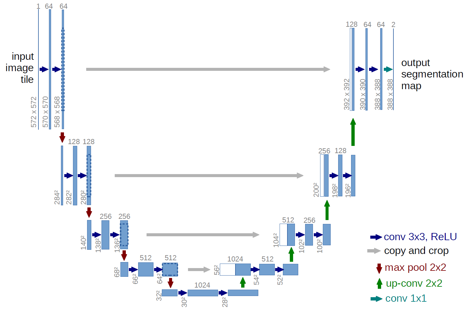
出典:
U-Net: Convolutional Networks for Biomedical Image Segmentation
U-Net: Convolutional Networks for Biomedical Image Segmentation
U-Netの実装
今回は,SegNetにスキップ構造を組み込んで性能比較(CaDIS: a Cataract Dataset)を参考にU-Netを構築しました.(CaDIS: a Cataract Datasetで画像セグメンテーションのSegNetにスキップ構造だけを導入したものです.)
import dataclasses
from tensorflow.keras.models import Model
from tensorflow.keras.layers import Input, MaxPool2D, UpSampling2D, concatenate
from tensorflow.keras.layers import Conv2D, BatchNormalization, Activation

# U-Net(エンコーダー8層、デコーダー8層)の構築
@dataclasses.dataclass
class U_NET:
    input_shape: tuple # 入力画像サイズ
    classes: int # 分類クラス数
    act_func: str # 活性化関数

    def __post_init__(self):
        # 入力画像サイズは32の倍数でなければならない
        assert self.input_shape[0]%32 == 0, 'Input size must be a multiple of 32.'
        assert self.input_shape[1]%32 == 0, 'Input size must be a multiple of 32.'

    # 活性化関数
    def activation(self, x):
        if self.act_func == 'relu':
            x = Activation('relu')(x)
        elif self.act_func == 'mish':
            x = Mish(x)
        elif self.act_func == 'frelu':
            x = FReLU(x)

        return x

    # エンコーダーブロック
    def encoder(self, x, blocks, filters, pooling):
        for i in range(blocks):
            x = Conv2D(filters, (3, 3), padding='same', kernel_initializer='he_normal')(x)
            x = BatchNormalization()(x)
            x = self.activation(x)

        if pooling:
            return MaxPool2D(pool_size=(2, 2))(x), x
        else:
            return x

    # デコーダーブロック
    def decoder(self, x1, x2, blocks, filters):
        x = UpSampling2D(size=(2, 2))(x1)
        x = concatenate([x, x2], axis=-1)

        for i in range(blocks):
            x = Conv2D(filters, (3, 3), padding='same', kernel_initializer='he_normal')(x)
            x = BatchNormalization()(x)
            x = self.activation(x)

        return x

    def create(self):
        # エンコーダー
        inputs = Input(shape=(self.input_shape[0], self.input_shape[1], 3)) # 入力層
        x, x1 = self.encoder(inputs, blocks=1, filters=32, pooling=True) # 1層目
        x, x2 = self.encoder(x, blocks=1, filters=64, pooling=True) # 2層目
        x, x3 = self.encoder(x, blocks=1, filters=128, pooling=True) # 3層目
        x, x4 = self.encoder(x, blocks=1, filters=256, pooling=True) # 4層目
        x, x5 = self.encoder(x, blocks=2, filters=512, pooling=True) # 5、6層目
        x = self.encoder(x, blocks=2, filters=1024, pooling=False) # 7、8層目

        # デコーダー
        x = self.encoder(x, blocks=1, filters=1024, pooling=False) # 1層目
        x = self.decoder(x, x5, blocks=2, filters=512) # 2、3層目
        x = self.decoder(x, x4, blocks=1, filters=256) # 4層目
        x = self.decoder(x, x3, blocks=1, filters=128) # 5層目
        x = self.decoder(x, x2, blocks=1, filters=64) # 6層目
        ## 7、8層目
        x = UpSampling2D(size=(2, 2))(x)
        x = concatenate([x, x1], axis=-1)
        x = Conv2D(64, (3, 3), strides=(1, 1), padding='same', kernel_initializer='he_normal')(x)
        x = Conv2D(self.classes, (1, 1), strides=(1, 1), padding='same', kernel_initializer='he_normal')(x)
        outputs = Activation('softmax')(x)

        return Model(inputs=inputs, outputs=outputs)
参考:SegNetにスキップ構造を組み込んで性能比較(CaDIS: a Cataract Dataset)
学習させる
それぞれの活性化関数で学習させていきます.
データセット準備
今回はデータセットとして以下を用います.
既存の公開データセットから選ばれた715枚の画像について,三種類のマスクデータがあるデータセットです.以下のPDFリンク
S. Gould, R. Fulton, D. Koller. Decomposing a Scene into Geometric and Semantically Consistent Regions. Proceedings of International Conference on Computer Vision (ICCV), 2009.
stanford background dataset をダウンロードおよび解凍します.
# ダウンロード
!wget http://dags.stanford.edu/data/iccv09Data.tar.gz

# 解凍
!tar -xzvf iccv09Data.tar.gz
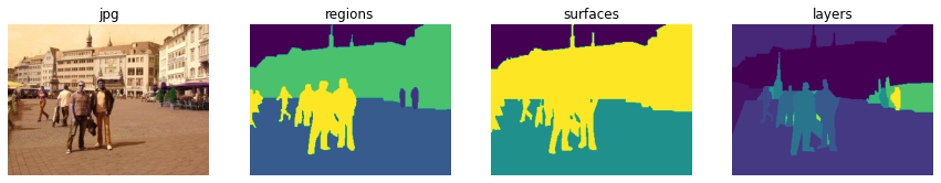
どんな画像があるか確認してみます.
import matplotlib.pyplot as plt
import numpy as np
import cv2

# どんな画像があるか確認
name = '0000047'                                                        # ファイル名を指定
img = cv2.imread(f'./iccv09Data/images/{name}.jpg')                     # jpg画像
label_regions = np.loadtxt(f'./iccv09Data/labels/{name}.regions.txt')   # 意味クラス(空, 木, 道, 草, 水, 建物, 山, 前景のオブジェクト)を示すマスク
label_surfaces = np.loadtxt(f'./iccv09Data/labels/{name}.surfaces.txt') # 幾何学的なクラス (空, 水平, 垂直) を示すマスク
label_layers = np.loadtxt(f'./iccv09Data/labels/{name}.layers.txt')     # 別々の画像領域を示すマスク

# 画像表示
display_list = [img, label_regions, label_surfaces, label_layers]
title = ['jpg', 'regions', 'surfaces', 'layers']
plt.figure(figsize=(15, 15))

for i in range(len(display_list)):
    plt.subplot(1, len(display_list), i+1)
    plt.title(title[i])
    plt.imshow(display_list[i])
    plt.axis('off')
plt.show()
結果は以下のようになります.
データセットを学習用に変換・分割
データセットを学習用に変換・分割します.正解ラベルの画像は、各クラスごとに画像を作成(クラス0であれば,元のマスク0の部分が1,それ以外は0の画像となるように)します.また,データは学習:検証:テスト = 6:2:2で分割します.
import glob
from keras.utils import generic_utils

# データセットの準備(label_typeでマスクを選択)
# label_type = 'regions' # 3クラス
label_type = 'surfaces' # 8クラス
# label_type = 'layers' # 調査予定

# 画像の一覧取得
images = sorted(glob.glob(f'./iccv09Data/images/*.jpg'))
labels = sorted(glob.glob(f'./iccv09Data/labels/*.{label_type}.txt'))

x = []
y = []
classes = 3                 # クラス数
ratio = 0.6                 # 学習データの割合 学習:検証:テスト = 6:2:2
input_shape = (224, 224)    # 32の倍数でないといけない

# 入力画像
for img_path in images:
    img = cv2.imread(img_path)
    img = cv2.resize(img, input_shape)      # 入力サイズに変換
    img = np.array(img, dtype=np.float32)   # float形に変換
    img *= 1./255                           # 0~1に正規化
    x.append(img)

# 正解ラベル
for label_path in labels:
    label = np.loadtxt(label_path)
    label = cv2.resize(label, input_shape)  # 入力サイズに変換
    img = []
    for label_index in range(classes):      # 各クラスごとに画像を作成(クラス0であれば、元のマスク0の部分が1、それ以外は0の画像となる)
        img.append(label == label_index)
    img = np.array(img, np.float32)         # float形に変換
    img = img.transpose(1, 2, 0)            # (クラス数, 224, 224) => (224, 224, クラス数)
    y.append(img)

x_data = np.array(x)
y_data = np.array(y)

# データを分割
p1 = int(ratio * len(x_data))
p2 = int((len(x_data) + p1) / 2) # len(x_data) - (len(x_data) - p1) / 2
x_train = x_data[:p1]
y_train = y_data[:p1]
x_val = x_data[p1:p2]
y_val = y_data[p1:p2]
x_test = x_data[p2:]
y_test = y_data[p2:]
y_test_label = labels[p2:] # 検証時にはラベル名から直接マスク取得するのでこちらを用意
学習
最適化関数や学習時のコールバックなどの設定を行い,モデル構築,学習を行います.
今回はそれぞれの関数についてregionsとsurfacesを対象に5回ずつ学習させました.
# 個別で学習
# label_type,input_shape,classesはデータ変換時に指定済み
activation_function = 'relu'
optimizer = Adam(lr=0.001, amsgrad=True) # 最適化関数

# 学習が停滞したとき、学習率を0.2倍に
rl_cb = ReduceLROnPlateau(monitor='loss', factor=0.2, patience=3,
                        verbose=1, mode='auto',
                        min_delta=0.0001, cooldown=0, min_lr=0)
# 学習が進まなくなったら、強制的に学習終了
es_cb = EarlyStopping(monitor='loss', min_delta=0,
                    patience=5, verbose=1, mode='auto')

# val_lossが最小になったときのみmodelを保存
mc_cb = ModelCheckpoint(f'model_weights_{activation_function}_{label_type}.h5',
                        monitor='val_loss', verbose=1,
                        save_best_only=True, mode='min')

# ネットワーク構築
model = U_NET(input_shape=input_shape, classes=classes, act_func=activation_function).create()
model.compile(optimizer=optimizer, loss='categorical_crossentropy', metrics=['accuracy'])

# 学習
history = model.fit(
    x=x_train,
    y=y_train,
    batch_size=16,
    epochs=100,
    verbose=1,
    callbacks=[mc_cb, rl_cb, es_cb],
    validation_data=(x_val, y_val)
)
# まとめて学習
activation_functions_list = ["relu", "mish", "frelu"]
times = 5

for activation_function in activation_functions_list:
    for i in range(times):
        optimizer = Adam(lr=0.001, amsgrad=True) # 最適化関数
        # 学習が停滞したとき、学習率を0.2倍に
        rl_cb = ReduceLROnPlateau(monitor='loss', factor=0.2, patience=3,
                                verbose=1, mode='auto',
                                min_delta=0.0001, cooldown=0, min_lr=0)
        # 学習が進まなくなったら、強制的に学習終了
        es_cb = EarlyStopping(monitor='loss', min_delta=0,
                            patience=5, verbose=1, mode='auto')
        # val_lossが最小になったときのみmodelを保存
        mc_cb = ModelCheckpoint(f'model_weights_{activation_function}_{label_type}_{i:03}.h5',
                                monitor='val_loss', verbose=1,
                                save_best_only=True, mode='min')

        # ネットワーク構築
        model = U_NET(input_shape=input_shape, classes=classes, activation_function=activation_function).create()
        model.compile(optimizer=optimizer, loss='categorical_crossentropy', metrics=['accuracy'])

        history = model.fit(
            x=x_train,
            y=y_train,
            batch_size=16,
            epochs=100,
            verbose=1,
            callbacks=[mc_cb, rl_cb, es_cb],
            validation_data=(x_val, y_val)
        )
参考:CaDIS: a Cataract Datasetで画像セグメンテーション
結果
学習したモデルそれぞれについて,クラスごとのaverage IoUとそれの平均を取ったmean IoUで評価をします.以下が評価用の関数です.
from collections import defaultdict

def calc_IoU(activation_function, label_type, model_num):
    model = U_NET(input_shape=input_shape, classes=classes, act_func=activation_function).create()
    model.load_weights(f'model_weights_{activation_function}_{label_type}_{model_num:03}.h5')
    # 推論
    dict_iou = defaultdict(list)
    for num in range(len(x_test)):
        input_img = x_test[num]                                             # 入力画像
        true_img = np.loadtxt(y_test_label[num])                            # 正解マスク
        height, width = true_img.shape[:2]                                  # 正解マスクのサイズ
        preds = model.predict(x_test[num][np.newaxis, ...])                 # 予測(長さ1の配列で渡す)
        pred_img = preds[0]

        pred_img = cv2.resize(pred_img, (width, height), interpolation=cv2.INTER_LANCZOS4)
        pred_img = np.argmax(pred_img, axis=2)
        ## IoUの計算
        for j in range(classes):
            y_pred = np.array(pred_img == j, dtype=np.int)
            y_true = np.array(true_img == j, dtype=np.int)
            tp = sum(sum(np.logical_and(y_pred, y_true)))
            other = sum(sum(np.logical_or(y_pred, y_true)))
            if other != 0:
                dict_iou[j].append(tp/other)

    # average IoU
    for i in range(classes):
        if i in dict_iou:
            dict_iou[i] = sum(dict_iou[i]) / len(dict_iou[i])
        else:
            dict_iou[i] = -1

    print(f'\n{activation_function}_{label_type}_{model_num:03}')
    dict_sum = 0
    for item in dict_iou:
        dict_sum += dict_iou[item]
        print(f"{(dict_iou[item] * 100):.5} %")

    print(f"\n{(dict_sum * 100 / classes):.5} %")
    dict_iou["mean_IoU"] = dict_sum / classes
    return dict_iou
参考:CaDIS: a Cataract Datasetで画像セグメンテーション
評価した結果,以下のようになりました(5回の平均と最大値).
surfaces
| 活性化関数 | mean IoU の平均 | mean IoU の最大 |
|---|---|---|
| ReLU | 76.8% | 77.3% |
| Mish | 78.2% | 78.8% |
| FReLU | 77.8% | 78.4% |
regions
| 活性化関数 | mean IoU の平均 | mean IoU の最大 |
|---|---|---|
| ReLU | 27.3% | 32.1% |
| Mish | 33.1% | 34.1% |
| FReLU | 32.9% | 33.9% |
結果としては,ReLUに比べてFReLUとMishの方が良い精度でした.
まとめ
今回はU-Netの活性化関数を変更してmean IoUで評価・比較しました.活性化関数を変えることで表現が変わることが確認できた気がします.データセットを変えたり,データ拡張したりしての学習やそれぞれの予測結果の比較などまだまだ詳しく調査できていないので,今後追記していきたいと思います.
追記
2020/02/24
FReLUに関しては,以下のツイートで精度向上の起因がどこにあるかを実験されていました.
https://twitter.com/AkiraTOSEI/status/1296774800128368641?s=20
「深くしたことが精度向上主要因で、DWCは精度/効率の両面で良さげ。設計による効果は薄そう」
という結果になっているので,今後U-Netでも同様の実装をして試してみたいと思います.
2020/03/03
@artemis5656 さんよりご指摘いただき,
FReLUのDepthwiseConv2Dにuse_bias=Falseを追加しました.
ありがとうございます!