機械学習 〜 線形モデル（分類） 〜

今回は scikit-learn の 線形モデルを使った分類を試してみます。

線形モデル（クラス分類）の予測式

線形モデルを使った分類の基本的な予測式は以下のようになります。

\hat{y} = \sum_{i=1}^{n} (w_{i}x_{i}) + b = w_1x_1 + w_2x_2 \cdots + w_nx_n + b > 0

予測された値が 0 より大きい値ならクラスA、0 以下ならクラスB といった形で分類を行います。

２クラス分類

2クラス分類を行います。

インポート

%matplotlib inline
import numpy as np
import pandas as pd
import matplotlib.pyplot as plt

from sklearn.model_selection import train_test_split
from sklearn.metrics import mean_squared_error
from sklearn.metrics import mean_absolute_error

２クラス用データ生成

make_classification クラスを使い、2クラス用のデータを生成します。

# データ生成
from sklearn.datasets import make_classification

X, Y = make_classification(random_state=12,
                           n_features=2, 
                           n_redundant=0, 
                           n_informative=1,
                           n_clusters_per_class=1,
                           n_classes=2)

fig = plt.figure()
plt.figure(figsize=(8, 7))
plt.title("make_classification : n_features=2  n_classes=2")
plt.scatter(X[:, 0], X[:, 1], marker='o', c=Y, s=25, edgecolor='k')
plt.xlabel("Feature 1")
plt.ylabel("Feature 2")

以下のようなデータ群が出力されます。

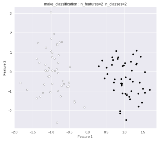
このデータを２クラス分類します。
まずは、パーセプトロンを使ってクラス分類を行います。

パーセプトロン

・神経回路を人工的にモデル化したもの
・複数の信号を入力として受け取り、１つの信号を出力
・線形分離可能なものしか学習できない

クラス

sklearn.linear_model.Perceptron クラスを使用します。

トレーニング・予測・評価

########################
# パーセプトロン
########################
from sklearn.linear_model import Perceptron

# トレーニング・テストデータ分割
X_train, X_test, Y_train, Y_test = train_test_split(X, Y, random_state=0)

# Perceptron
ppt = Perceptron()
ppt.fit(X_train, Y_train)

# 予測　
Y_pred = ppt.predict(X_test)

#
# 評価
#
# 平均絶対誤差(MAE)
mae = mean_absolute_error(Y_test, Y_pred)
# 平方根平均二乗誤差（RMSE）
rmse = np.sqrt(mean_squared_error(Y_test, Y_pred))
# スコア
score = ppt.score(X_test, Y_test)

coef = ppt.coef_[0]
intercept = ppt.intercept_

print("MAE = %.3f,  RMSE = %.3f,  score = %.3f" % (mae, rmse, score))
print("Coef =", coef)
print("Intercept =", intercept)

MAE = 0.000,  RMSE = 0.000,  score = 1.000
Coef = [3.3300988  0.79334844]
Intercept = [-1.]

プロット

# プロット
plt.figure(figsize=(8, 7))
plt.scatter(X[:, 0], X[:, 1], marker='o', c=Y, s=25, edgecolor='k')

line = np.linspace(-15, 15)
plt.plot(line, -(line * coef[0] + intercept) / coef[1], c='g', label="Perceptron")
plt.ylim(-2.9, 3.4)
plt.xlim(-2, 1.8)
plt.legend()

クラスを分ける決定境界が表示されました。

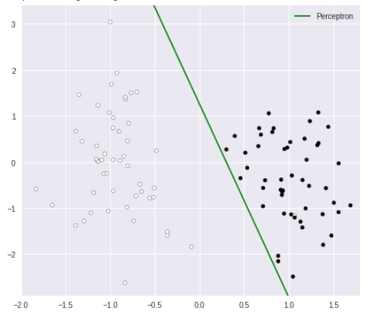
次に、ロジスティック回帰を使ってクラス分類を行ってみます。

ロジスティック回帰

・シグモイド関数（ロジスティック関数）を使い 0〜１の数値を信頼度として出力
・パラメータの更新には確率的勾配降下法（SGD:stochastic gradient descent）を利用
・http://gihyo.jp/dev/serial/01/machine-learning/0018

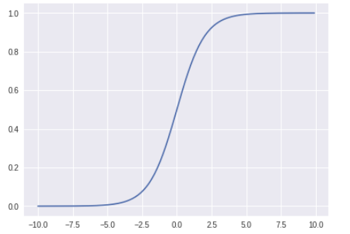
シグモイド関数

・0〜１の数値を出力
・x の値が大きくなるにつれ、出力値が 1 に近づく
・x の値が小さくなるにつれ、出力値が 0 に近づく

式は以下の通り

f(x) = \frac{1}{1+exp(-x)}

クラス

sklearn.linear_model.LogisticRegression クラスを使用します。

引数（一部）

パラメータ名	概要	備考
penalty	正則化	‘l1’ : L1正則化 ‘l2’ : L2正則化（初期値）
C	正則化項のハイパーパラメータ	（初期値:1.0）
solver	最適化問題で使用するアルゴリズム	‘newton-cg’：ニュートン法 ‘lbfgs’：L-BFGSアルゴリズム ‘liblinear’：（初期値） ‘sag’：Stochastic Average Gradient ‘saga：A Fast Incremental Gradient Method with Support for Non-Strongly Convex Composite Objectives

※SAG, SAGA は SGD の改良版

トレーニング・予測・評価

今回は、最適化アルゴリズムに ‘sag’ を使用します。

########################
# ロジスティック回帰
########################
from sklearn.linear_model import LogisticRegression

# トレーニング・テストデータ分割
X_train, X_test, Y_train, Y_test = train_test_split(X, Y, random_state=0)

# LogisticRegression
logreg = LogisticRegression(penalty='l2', solver="sag")
logreg.fit(X_train, Y_train)

# 予測　
Y_pred = logreg.predict(X_test)

#
# 評価
#
# 平均絶対誤差(MAE)
mae = mean_absolute_error(Y_test, Y_pred)
# 平方根平均二乗誤差（RMSE）
rmse = np.sqrt(mean_squared_error(Y_test, Y_pred))
# スコア
score = logreg.score(X_test, Y_test)

coef = logreg.coef_[0]
intercept = logreg.intercept_

print("MAE = %.3f,  RMSE = %.3f,  score = %.3f" % (mae, rmse, score))
print("Coef =", coef)
print("Intercept =", intercept)

MAE = 0.000,  RMSE = 0.000,  score = 1.000
Coef = [3.05571024 0.27793757]
Intercept = [-0.32060796]

プロット

# プロット
plt.figure(figsize=(8, 7))
plt.scatter(X[:, 0], X[:, 1], marker='o', c=Y, s=25, edgecolor='k')

line = np.linspace(-15, 15)
plt.plot(line, -(line * coef[0] + intercept) / coef[1], c='r', label="LogisticRegression")
plt.ylim(-2.9, 3.4)
plt.xlim(-2, 1.8)
plt.legend()

クラスを分ける決定境界が表示されました。

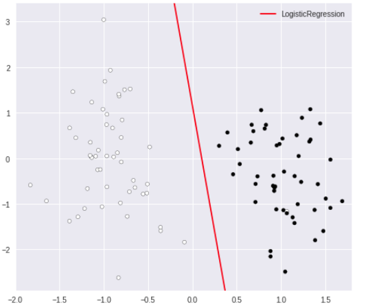
次に、SVM（サポートベクターマシン）を使ってクラス分類を行ってみます。

SVM（サポートベクターマシン）

・決定境界線とデータとの最短距離を最大化するマージン最大化という手法を使う
・カーネルトリックを使い、線形分離不可能な場合でも適用可能

クラス

sklearn.svm.LinearSVC クラスを使用します。

引数（一部）

パラメータ名	概要	備考
penalty	正則化	‘l1’ : L1正則化 ‘l2’ : L2正則化（初期値）
C	正則化項のハイパーパラメータ	（初期値:1.0）

トレーニング・予測・評価

########################
# LinearSVC
########################
from sklearn.svm import LinearSVC

# トレーニング・テストデータ分割
X_train, X_test, Y_train, Y_test = train_test_split(X, Y, random_state=0)

# LinearSVC
linear_svc = LinearSVC()
linear_svc.fit(X_train, Y_train)

# 予測　
Y_pred = linear_svc.predict(X_test)

# 評価
score = linear_svc.score(X_test, Y_test)

coef = linear_svc.coef_[0]
intercept = linear_svc.intercept_

print("score = %.3f" % (score))
print("Coef =", coef)
print("Intercept =", intercept)

score = 1.000
Coef = [1.37856834 0.22061591]
Intercept = [-0.11932797]

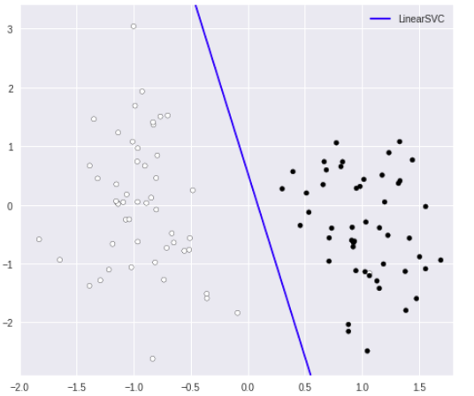
プロット

# プロット
plt.figure(figsize=(8, 7))
plt.scatter(X[:, 0], X[:, 1], marker='o', c=Y, s=25, edgecolor='k')

line = np.linspace(-15, 15)
plt.plot(line, -(line * coef[0] + intercept) / coef[1], c='b', label="LinearSVC")
plt.ylim(-2.9, 3.4)
plt.xlim(-2, 1.8)
plt.legend()

多クラス分類

次に多クラス分類を行います。

多クラス用データ生成

まずは、make_blobs クラスを使い
３クラスに分類されたデータを生成します。

# データ生成
####################################
# ３クラス分類
####################################
from sklearn.datasets import make_blobs
X, Y = make_blobs(random_state=10)

print("X =", X[:3])
print("Y =", Y[:20])

plt.figure(figsize=(8, 7))
plt.title("make_classification : n_features=2  n_classes=3")
plt.scatter(X[:, 0], X[:, 1], marker='o', c=Y, s=25, edgecolor='k')
plt.xlabel("Feature 1")
plt.ylabel("Feature 2")

X = [[-2.32496308 -6.6999964 ]
 [ 0.51856831 -4.90086804]
 [ 2.44301805  3.84652646]]
Y = [2 2 1 0 1 1 0 2 1 0 0 1 1 2 2 1 0 1 0 1]

以下のようなデータ群が出力されます。

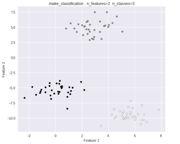
このデータを多クラス分類します。
分類領域のプロット関数を先に定義しておきます。

# 分類領域プロット
def plot_2d_classification(model, X, margin=1):
    # 最大・最小値
    x_min, x_max = X[:, 0].min() - margin, X[:, 0].max() + margin
    y_min, y_max = X[:, 1].min() - margin, X[:, 1].max() + margin
    # 等間隔な数列生成
    ls_x = np.linspace(x_min, x_max, 1000)
    ls_y = np.linspace(y_min, y_max, 1000)
    # グリッド生成
    g_x, g_y = np.meshgrid(ls_x, ls_y)
    grid_X = np.c_[g_x.ravel(), g_y.ravel()]
    # 予測    
    z = model.predict(grid_X)
    z = z.reshape(g_x.shape)
    # プロット
    cmap = ListedColormap(('red', 'blue', 'green'))
    plt.contourf(g_x, g_y, z, alpha=0.4, cmap=cmap)
    plt.xlim(x_min, x_max)
    plt.ylim(y_min, y_max)

まずは、パーセプトロンを使ってクラス分類してみます。

パーセプトロン

トレーニング・予測・評価

########################
# パーセプトロン
########################
from sklearn.linear_model import Perceptron

# トレーニング・テストデータ分割
X_train, X_test, Y_train, Y_test = train_test_split(X, Y, random_state=0)

# Perceptron
ppt = Perceptron()
ppt.fit(X_train, Y_train)

# 予測　
Y_pred = ppt.predict(X_test)

#
# 評価
#
# 平均絶対誤差(MAE)
mae = mean_absolute_error(Y_test, Y_pred)
# 平方根平均二乗誤差（RMSE）
rmse = np.sqrt(mean_squared_error(Y_test, Y_pred))
# スコア
score = ppt.score(X_test, Y_test)

coef = ppt.coef_
intercept = ppt.intercept_

print("MAE = %.3f,  RMSE = %.3f,  score = %.3f" % (mae, rmse, score))
print("Coef =", coef)
print("Intercept =", intercept)

MAE = 0.160,  RMSE = 0.566,  score = 0.920
Coef = [[  4.85315786  -0.92354112]
 [  0.26686394   5.44678194]
 [-30.56260373  -1.33073394]]
Intercept = [-22.  -1.   7.]

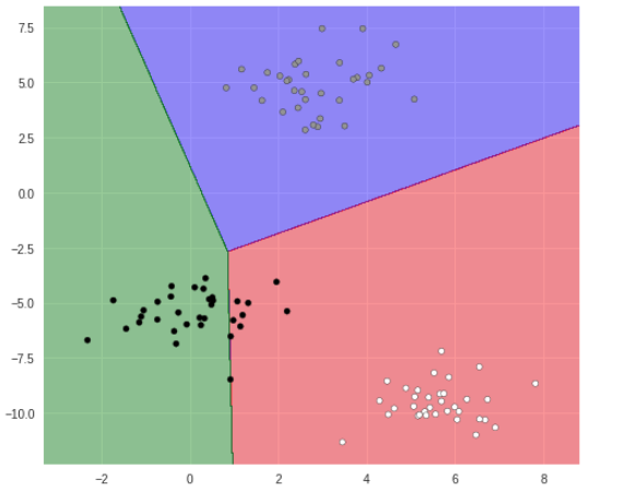
プロット

# 分類領域プロット
plt.figure(figsize=(8, 7))
plot_2d_classification(ppt, X)
plt.scatter(X[:, 0], X[:, 1], marker='o', c=Y, s=25, edgecolor='k')

黒丸の分類が上手く行えていないようです。

ロジスティック回帰

トレーニング・予測・評価

########################
# ロジスティック回帰
########################
from sklearn.linear_model import LogisticRegression

# トレーニング・テストデータ分割
X_train, X_test, Y_train, Y_test = train_test_split(X, Y, random_state=0)

# LogisticRegression
logreg = LogisticRegression(penalty='l2', solver="sag")
logreg.fit(X_train, Y_train)

# 予測　
Y_pred = logreg.predict(X_test)

#
# 評価
#
# 平均絶対誤差(MAE)
mae = mean_absolute_error(Y_test, Y_pred)
# 平方根平均二乗誤差（RMSE）
rmse = np.sqrt(mean_squared_error(Y_test, Y_pred))
# スコア
score = logreg.score(X_test, Y_test)

coef = logreg.coef_
intercept = logreg.intercept_

print("MAE = %.3f,  RMSE = %.3f,  score = %.3f" % (mae, rmse, score))
print("Coef =", coef)
print("Intercept =", intercept)

MAE = 0.000,  RMSE = 0.000,  score = 1.000
Coef = [[ 1.06810974 -0.46558499]
 [ 0.26397664  1.08209724]
 [-1.92862092 -0.42300224]]
Intercept = [-6.3464851  -0.02418883  2.05724535]

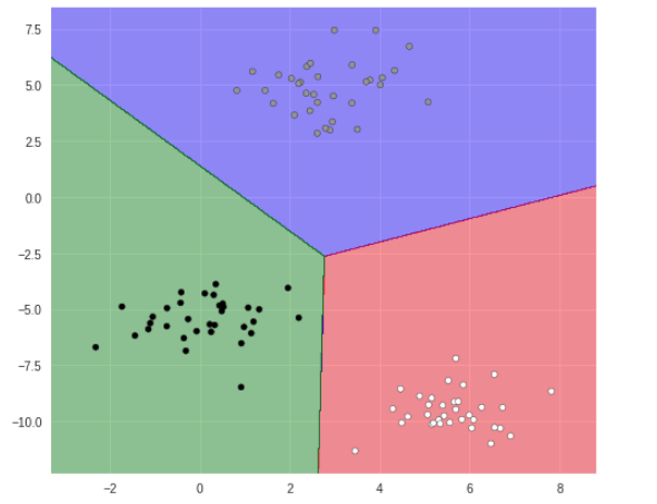
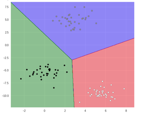
プロット

# 分類領域プロット
plt.figure(figsize=(8, 7))
plot_2d_classification(logreg, X)
plt.scatter(X[:, 0], X[:, 1], marker='o', c=Y, s=25, edgecolor='k')

上手く分類されています。

SVM（サポートベクターマシン）

トレーニング・予測・評価

########################
# LinearSVC
########################
from sklearn.svm import LinearSVC

# トレーニング・テストデータ分割
X_train, X_test, Y_train, Y_test = train_test_split(X, Y, random_state=0)

# LinearSVC
linear_svc = LinearSVC()
linear_svc.fit(X_train, Y_train)

# 予測　
Y_pred = linear_svc.predict(X_test)

# 評価
score = linear_svc.score(X_test, Y_test)

coef = linear_svc.coef_
intercept = linear_svc.intercept_

print("score = %.3f" % (score))
print("Coef =", coef)
print("Intercept =", intercept)

score = 1.000
Coef = [[ 0.35131054 -0.12909795]
 [ 0.06475561  0.27764857]
 [-0.75515781 -0.15512279]]
Intercept = [-1.97518937  0.01648068  0.92792459]

プロット

# 分類領域プロット
plt.figure(figsize=(8, 7))
plot_2d_classification(linear_svc, X)
plt.scatter(X[:, 0], X[:, 1], marker='o', c=Y, s=25, edgecolor='k')

こちらも上手く分類されています。

以上、scikit-learn の 線形モデルを使った分類を試してみました。